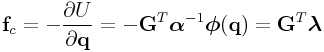
May 10, 2012
0.1 Spatial Inertia Matrices
Given a rigid body with mass ![]() , center of mass
, center of mass ![]() (with respect
to body coordinates), and rotational inertia
(with respect
to body coordinates), and rotational inertia ![]() (with respect
to the center of mass), then the
(with respect
to the center of mass), then the ![]() spatial inertia matrix
is given by
spatial inertia matrix
is given by
![{\bf M}=\left(\begin{matrix}m{\bf I}&-m[{\bf c}]\\
m[{\bf c}]&{\bf J}-m[{\bf c}][{\bf c}]\end{matrix}\right)](mi/mi282.png) |
where ![]() denotes the
denotes the ![]() skew-symmetric cross product matrix
of
skew-symmetric cross product matrix
of ![]() . The inverse is given by
. The inverse is given by
![{\bf M}^{{-1}}=\left(\begin{matrix}\frac{1}{m}{\bf I}-[{\bf c}]{\bf J}^{{-1}}[{\bf c}]&[{\bf c}]{\bf J}^{{-1}}\\
-{\bf J}^{{-1}}[{\bf c}]&{\bf J}^{{-1}}\end{matrix}\right)](mi/mi286.png) |
Note that this factors into ![]() , with
, with
![{\bf G}=\left(\begin{matrix}\sqrt{m}{\bf I}&0\\
\sqrt{m}[{\bf c}]&{\bf L}\end{matrix}\right)](mi/mi264.png) |
and ![]() .
.
0.2 Quaternions
A rotation consisting of a rotation ![]() about an axis
about an axis ![]() is
described by a unit quarternion
is
described by a unit quarternion ![]() according to
according to
Given two quaterions ![]() and
and ![]() , with scalar components
, with scalar components ![]() and
and
![]() and vector components
and vector components ![]() and
and ![]() , the product
, the product ![]() is
defined by
is
defined by
Given an angular velocity ![]() in base coordinates, the time
derivative of a unit quaternion
in base coordinates, the time
derivative of a unit quaternion ![]() is given by
is given by
| (0.1) |
with ![]() denoting a quaternion with zero scalar component
and a vector component of
denoting a quaternion with zero scalar component
and a vector component of ![]() . If the angular velocity is
instead given in the rotated coordinate system, then
. If the angular velocity is
instead given in the rotated coordinate system, then
If a quaternion represents a rotated coordinate system, then
the transformation of a vector ![]() from rotated to world
coordinates is given by
from rotated to world
coordinates is given by
0.3 Equivalence between LCP and Quadratic Programming
A quadratic program which calls for us to minimize
with ![]() SPD, is equivalent to the LCP
SPD, is equivalent to the LCP
where
0.4 Derivatives of roll, pitch and yaw angles
Spherical joints in ArtiSynth can be controlled using roll-pitch-yaw
angles ![]() ,
, ![]() ,
, ![]() , in which an orientation is obtained by
a rotation of
, in which an orientation is obtained by
a rotation of ![]() about the
about the ![]() axis, followed by a rotation of
axis, followed by a rotation of
![]() about the new
about the new ![]() axis, followed by a rotation of
axis, followed by a rotation of ![]() about
the final
about
the final ![]() axis.
axis.
The total angular velocity ![]() can be expressed in terms of the
can be expressed in terms of the
![]() ,
, ![]() and
and ![]() according to
according to
Representing everything in terms of the orginal base frame, this leads to
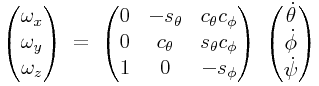 |
where ![]() ,
, ![]() ,
, ![]() , and
, and ![]() are the cosines and sines
of
are the cosines and sines
of ![]() and
and ![]() .
Inverting this relationship, we obtain
.
Inverting this relationship, we obtain
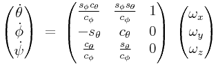 |
(0.2) |
Note that there is a singularity when ![]() , since this
implies alignment of the
, since this
implies alignment of the ![]() and
and ![]() axes.
axes.
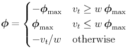
When implementing joint limit constraints for the ![]() ,
, ![]() and
and
![]() angles, the corresponding constraint wrenches are
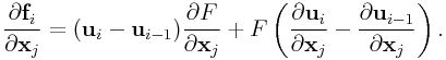
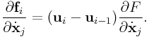
formed by the rows of (0.2). The derivatives
of these rows are given by
angles, the corresponding constraint wrenches are
formed by the rows of (0.2). The derivatives
of these rows are given by
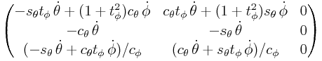 |
where ![]() .
.
0.5 Constraint Satisfaction as Projection
Assume we have a mechanical system with a mass matrix ![]() , a
state vector
, a
state vector ![]() , applied forces
, applied forces ![]() , and a matrix of
contraints
, and a matrix of
contraints ![]() such that
such that
The corresponding constraint forces then lie in the range of ![]() ,
and are computed such that
,
and are computed such that
This implies that
and so the constrained force ![]() is given by
is given by
or
where
Similarly, we can ensure that velocity constraints are satisfied by
applying an impulse ![]() , so that
the constrained velocity
, so that
the constrained velocity ![]() is given by
is given by
or
where
It is easy to show that
When constraints are expressed in the form of a KKT system, we can also show that
 |
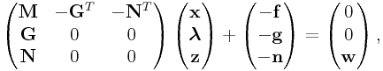
0.6 Solution of a general KKT system
Given a KKT system
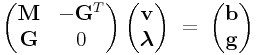 |
(0.3) |
we have that
In terms of the projection matrices of the previous section, we have
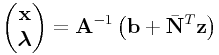
0.7 Turning a mixed LCP into a regular LCP
Assume the following mixed LCP:
We can turn this into a pure LCP by solving for ![]()
and then subsituting this into ![]() :
:
In terms of the projection ![]() described in the previous section,
this can be expressed as
described in the previous section,
this can be expressed as
which if ![]() reduces to
reduces to
If the mixed LCP is expressed as
 |
||
then we can partition this into
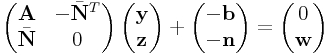 |
with
 |
and create a regular LCP from
This will require ![]() solves of
solves of ![]() , where
, where ![]() is the number of
rows of
is the number of
rows of ![]() . Once we have solved for
. Once we have solved for ![]() , we can
back solve for
, we can
back solve for ![]() and
and ![]() from
from
 |
0.8 On demand pivoting for a mixed LCP formulation
The matrix ![]() described in the previous section can be created on demand, which
may be advantageous if the number of pivots is smaller that
the number of columns of
described in the previous section can be created on demand, which
may be advantageous if the number of pivots is smaller that
the number of columns of ![]() .
.
For principal pivoting algorithms, the
LCP matrix ![]() and constant vector
and constant vector ![]() are partitioned into
are partitioned into
 |
with their pivoted versions given by
 |
(0.4) |
The on-demand scheme works as follows. Column ![]() of
of ![]() is
computed (and stored) whenever
is
computed (and stored) whenever ![]() is added to the basis for the
first time. This means that we always have
is added to the basis for the
first time. This means that we always have ![]() and
and ![]() available, with a factorization of the former maintained so that we
can easily compute products of
available, with a factorization of the former maintained so that we
can easily compute products of ![]() .
.
Pivoting algorithms require ![]() and the
and the ![]() -th column of
-th column of ![]() ,
which we denote by
,
which we denote by ![]() .
The former can be determined using
.
The former can be determined using ![]() and
and ![]() , assuming that
, assuming that ![]() has already been computed, as per (0.4).
For
has already been computed, as per (0.4).
For ![]() , if
, if ![]() , then
we have
, then
we have
 |
Otherwise, if ![]() , we compute
, we compute ![]() if necessary,
and then
if necessary,
and then
 |
0.9 Solvers
Given a mechanical system defined by a mass matrix ![]() , state
, state
![]() , and applied force
, and applied force ![]() , we can
solve for its time evolution using several integrator types:
, we can
solve for its time evolution using several integrator types:
0.9.1 Symplectic Euler:
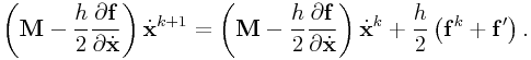
0.9.2 Implicit Euler:
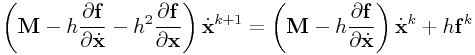 |
The velocity expression can be expressed as
where
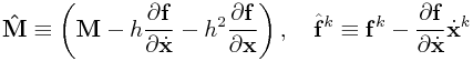 |
or as
with
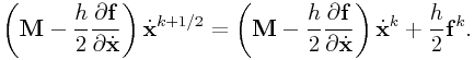
0.9.3 Trapezoidal:
For the trapezoidal rule, we determine ![]() from
from
which leads to
 |
Again, the velocity expression can be expressed as
where
 |
or as
with
0.9.4 Bridson-Marino:
This involves first computing an intermediate velocity ![]() :
:
 |
![]() is now modified to satisfy constraints,
and from this we compute
is now modified to satisfy constraints,
and from this we compute ![]() :
:
We can then determine ![]() , and use this to
solve for
, and use this to
solve for ![]() :
:
 |
Note that the position Jacobian is not used.
0.10 Integration with Constraints
Adding bilateral constraints ![]() and unilateral constraints
and unilateral constraints
![]() to the above systems, we obtain
to the above systems, we obtain
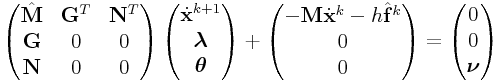 |
||
If we add box friction to the system, we obtain
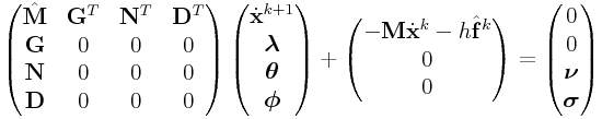 |
(0.5) | ||
| (0.6) |
where ![]() and
and ![]() are box bounds on
are box bounds on ![]() determined from the friction coefficients
determined from the friction coefficients ![]() and an estimate of
and an estimate of
![]() .
.
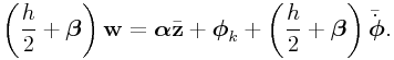
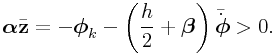
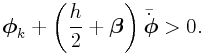
If we wish Anitescu/Stewart friction, then we obtain a more elaborate system
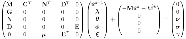 |
||
The matrix ![]() is defined such that
is defined such that ![]() for all
for all
![]() corresponding to the frictional wrenches
corresponding to the frictional wrenches ![]() of the same
contact. It enforces the friction cone and maximal dissipation
constraints: for a given contact with friction wrenches
of the same
contact. It enforces the friction cone and maximal dissipation
constraints: for a given contact with friction wrenches ![]() ,
we have
,
we have
![\mu\theta-\sum\phi _{k}=\gamma=\left\{\begin{array}[]{ll}=0&\mbox{on the friction cone}\\
>0&\mbox{inside the friction cone}\end{array}\right.](mi/mi251.png) |
![{\bf d}_{k}{\bf v}+\xi=\sigma=\left\{\begin{array}[]{ll}=0&\mbox{if ${\bf d}_{k}{\bf v}$ is maximally negative}\\
>0&\mbox{if ${\bf d}_{k}{\bf v}$ is {\it not} maximally negative}\end{array}\right.](mi/mi329.png) |
Then from the friction cone constraint we have
and from maximal dissiption we get
0.11 Softening Constraints with Regularization
This material uses ideas from [].
Consider a general KKT system such as that described by
(0.3), and let ![]() denote the constraint function
for which
denote the constraint function
for which ![]() is the derivative.
is the derivative.
Instead of enforcing constraints exactly, we can enforce them using a
potential function based on the distance from the constraint (defined
by ![]() ), such as
), such as
where ![]() is an inverse stiffness matrix. The constraint
forces
is an inverse stiffness matrix. The constraint
forces ![]() arising from this are given by
arising from this are given by
 |
where ![]() now gives the “soft” constraint
force. We can also add a damping term
now gives the “soft” constraint
force. We can also add a damping term ![]() , so that
, so that
| (0.7) |
(Note that here the full damping term is ![]() ).
).
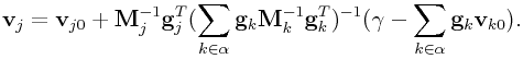
Now we will integrate (0.7) into a KKT system where
we are solving for updated velocity values ![]() . Following the
derivation in [], we consider the average
value
. Following the
derivation in [], we consider the average
value ![]() of
of ![]() over the time step, or more specifically,
over the time step, or more specifically,
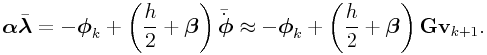
Using the approximations ![]() ,
,
![]() , and finally
, and finally
![]() , where
, where ![]() is
the step size, we obtain
is
the step size, we obtain
 |
(0.8) |
Now defining ![]() , we can rearrange this
as
, we can rearrange this
as
where ![]() denotes the constraint impulse we
which to solve for along with
denotes the constraint impulse we
which to solve for along with ![]() . This fits into a
KKT framework as
. This fits into a
KKT framework as
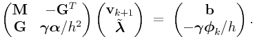 |
(0.9) |
Note in particular that if ![]() , then
, then ![]() , and so
, and so
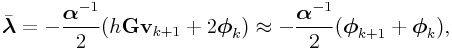 |
implying that ![]() is approximatelty equal to the average value
of
is approximatelty equal to the average value
of ![]() during the step, times the restoring stiffness.
during the step, times the restoring stiffness.
It is also possible to add regularization to unilateral constraints,
 |
(0.10) |
with ![]() denoting the unilateral constraint impulse
and
denoting the unilateral constraint impulse
and ![]() denoting the average constraint force.
To understand how this will behave, we
work backwards toward the form of (0.8) to obtain
denoting the average constraint force.
To understand how this will behave, we
work backwards toward the form of (0.8) to obtain
 |
Now, by the complementarity conditions, if ![]() , then
, then ![]() and so
and so
 |
Otherwise, if ![]() , then
, then ![]() and so
and so
 |
Note that for unilateral constraints, the damping term might introduce
some anomolous results. If ![]() and
and ![]() are both
negative, then
are both
negative, then ![]() , while if they are both positive, then
, while if they are both positive, then ![]() , as we would expect. However, if
, as we would expect. However, if ![]() and
and ![]() ,
then a large value of
,
then a large value of ![]() can cause
can cause ![]() even if the
interpenetration continues (i.e.,
even if the
interpenetration continues (i.e., ![]() ) at the end of the
time step.
) at the end of the
time step.
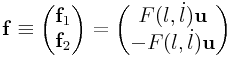
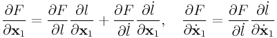
0.12 Jacobians for Axial Springs
An axial spring between two points ![]() and
and ![]() exerts forces
exerts forces ![]() and
and ![]() onto the points given by
onto the points given by
 |
where ![]() is a scalar describing the
spring force and
is a scalar describing the
spring force and
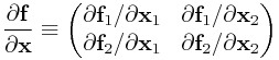
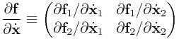
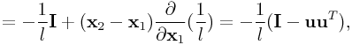
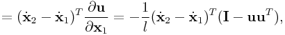
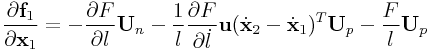
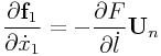
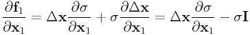
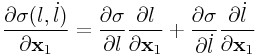
Differentiating this relationship with respect to node positions and velocities gives the position and velocity Jacobians:
 |
 |
Because of symmetry, it is easy to show that
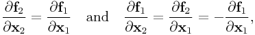 |
and similarly for the velocity Jacobian, and so it is sufficient to
analyze ![]() and
and
![]() .
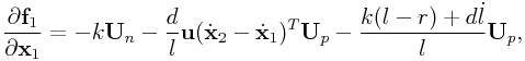
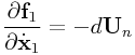
Applying the product rule to these gives
.
Applying the product rule to these gives
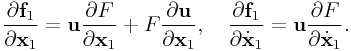 |
Applying the chain rule to ![]() gives
gives
 |
To continue our analysis, we utilize the following:
 |
|||
 |
|||
Then if we define ![]() and
and ![]() (which are the matrices that project a vector onto the direction of
(which are the matrices that project a vector onto the direction of
![]() and the plane perpendicular to
and the plane perpendicular to ![]() , respectively), and
assume that
, respectively), and
assume that ![]() and
and ![]() are given, we obtain
are given, we obtain
 |
 |
0.12.1 Linear Axial Springs
For a linear axial spring, we have
where ![]() and
and ![]() are the stiffness and damping coefficients,
and
are the stiffness and damping coefficients,
and ![]() is the rest lenth. Then
is the rest lenth. Then
 |
and
 |
||
 |
If ![]() , this reduces to
, this reduces to
 |
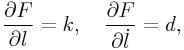
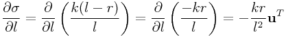
0.13 Spring Jacobians Formulated using Stress
If we reformulate the results of Section 0.12
using force-per-length, which we will call a “stress” ![]() defined by
defined by
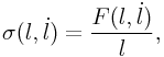 |
then we can replace the expression ![]() with
with
where ![]() . This approach is closer
to the finite element formulation for a two-element truss node
and can simplify the Jacobian calculations.
. This approach is closer
to the finite element formulation for a two-element truss node
and can simplify the Jacobian calculations.
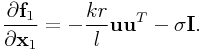
In particular, we now have
 |
Similar to before, we have
 |
If there is no dependence on ![]() , and
, and ![]() is linear so that
is linear so that
then
 |
and so
![]() reduces to
reduces to
 |
If the rest length ![]() is zero, then we have the very simple result
is zero, then we have the very simple result
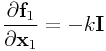 |
which is consistent with Section 0.12.1.
Most FEM formulations use a non-zero rest length, consistent with
having a finite size reference element. If we define a quadratic
strain ![]() by
by
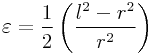 |
and relate this linearly to ![]() using
using
then we can show that
 |
and so
 |
In FEM parlance, the first term is the material stiffness, while the second term is the geometric stiffness.
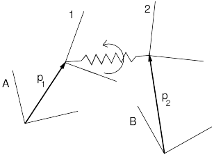
0.14 Jacobians for Multi-Point Springs
A multi-point spring is an axial spring with extra via points
that act like generalized pulleys and alter the spring’s direction
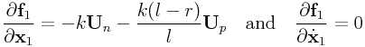
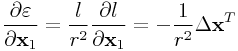
(Figure 0.1). The tension ![]() within the spring
is a function of the entire length
within the spring
is a function of the entire length ![]() and length derivative
and length derivative ![]() .
.
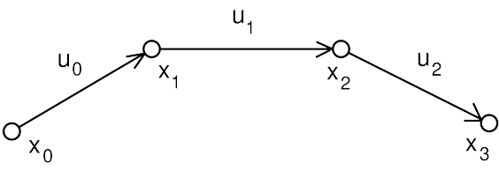
For the following discussion, we will assume that a multi-spring is
composed of ![]() segments, defined by
segments, defined by ![]() points
points ![]() , where
, where ![]() and
and ![]() are the end points and the
remaining
are the end points and the
remaining ![]() are the via points. The segments are associated with
direction vectors
are the via points. The segments are associated with
direction vectors ![]() and lengths
and lengths ![]() , defined by
, defined by
| (0.11) |
The forces on the end points and via points are given by
and the total length ![]() and its derivative is given by
and its derivative is given by
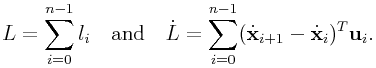 |
(0.12) |
Following the discussion of Section 0.12, we then have, for a via point,
 |
From (0.11), it can be determined that
for ![]() and
and ![]() we have
we have
 |
(0.13) |
where ![]() .
For
.
For ![]() , we have simply
, we have simply
 |
Because ![]() is a function of
is a function of ![]() and
and ![]() , it is affected by the
position and velocity of each point. In particular,
from the discussion of Section 0.12, we have
, it is affected by the
position and velocity of each point. In particular,
from the discussion of Section 0.12, we have
 |
From (0.12), we can determine
![]() ,
, ![]() ,
and
,
and ![]() :
:
 |
|||
 |
|||
More generally, for multi-point springs, we can define the notion of
active segments, which contribute to ![]() and
and ![]() , and passive segments, which do not. Let the set of active segments be
denoted by
, and passive segments, which do not. Let the set of active segments be
denoted by ![]() , and for notational convenience, consider
the endpoints
, and for notational convenience, consider
the endpoints ![]() and
and ![]() to be connected to fictitous
passive segments
to be connected to fictitous
passive segments ![]() and
and ![]() , respectively.
The
, respectively.
The ![]() and
and ![]() are then redefined by
are then redefined by
 |
(0.14) |
Now if we define ![]() such that
such that
then for all ![]() ,
,
and it is also straightforward to show that
 |
Moreover, if for ![]() we define
we define
 |
and ![]() otherwise, then
otherwise, then
 |
Then then leads to
 |
and
 |
where ![]() is given by (0.13).
is given by (0.13).
0.15 Gauss Seidel and KKT Systems
Consider a KKT system defined by
Solving this requires solving for ![]() according to
according to
| (0.15) |
Now, as described in Wikipedia, Gauss Seidel involves
solving ![]() by decomposing
by decomposing ![]() into
into ![]() , where
, where
![]() and
and ![]() are strictly lower and upper triangular, and then
applying the iteration
are strictly lower and upper triangular, and then
applying the iteration
| (0.16) |
Component-wise, this takes the form
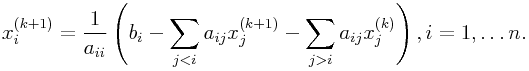 |
(0.17) |
Applying this to (0.15) gives
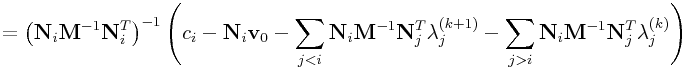 |
|||
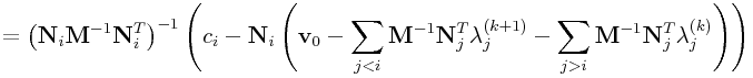 |
|||
where ![]() is the total velocity updated for the
is the total velocity updated for the ![]() -th
iteration step. The term
-th
iteration step. The term ![]() represents the
solution of constraint
represents the
solution of constraint ![]() in isolation; this term will be a scalar if
the constraints are all one-dimensional.
in isolation; this term will be a scalar if
the constraints are all one-dimensional.
0.16 A Gauss Seidel Friction Iteration
We describe here a Gauss-Seidel step to handle friction at a single
contact point. Assume that the constraint directions for this point
are given by ![]() (which in general, will be a
(which in general, will be a ![]() sparse
matrix, where each row is generated by the two tangential degrees of
freedom at the contact point, mapped onto the dynamic components
associated with the contact).
sparse
matrix, where each row is generated by the two tangential degrees of
freedom at the contact point, mapped onto the dynamic components
associated with the contact).
The tangential velocity components ![]() are then given by
are then given by
In response, a friction impulse ![]() is applied to
is applied to ![]() ,
resulting in a change in tangential velocity given by
,
resulting in a change in tangential velocity given by
Assuming that the size of the normal impulse ![]() is known, then
the maximum possible magnitude of the friction impulse is
is known, then
the maximum possible magnitude of the friction impulse is
![]() , where
, where ![]() is the friction
coefficient. The friction impulse
is the friction
coefficient. The friction impulse ![]() is applied to reduce
is applied to reduce
![]() as mush as possible given this limit:
as mush as possible given this limit:
 |
This is equivalent to the box friction conditions described in (0.6).
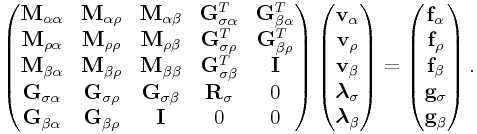
0.17 Null-space reduction of the KKT system for attachments
A component ![]() is attached to one or more active master components if its velocity can be directly determined from its
masters:
is attached to one or more active master components if its velocity can be directly determined from its
masters:
| (0.18) |
where ![]() is the attached component’s velocity, and
is the attached component’s velocity, and ![]() is
the velocity of all the active components.
is
the velocity of all the active components. ![]() will be
sparse except for entries corresponding to the master components to
which
will be
sparse except for entries corresponding to the master components to
which ![]() is attached.
is attached.
Let the set of active components be denoted by ![]() , and the set
of attached points be denoted by
, and the set
of attached points be denoted by ![]() .
Letting
.
Letting ![]() denote the matrix formed from
denote the matrix formed from ![]() for all
components, we have
for all
components, we have
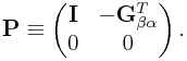
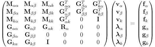
as the constraint that enforces all attachments. Adding this to the KKT system, and partitioning that system into attached components and active components, yields
 |
(0.19) |
where ![]() is a diagonal regularization matrix for the constraints
(since attachments are hard constraints, no regularization is
included).
is a diagonal regularization matrix for the constraints
(since attachments are hard constraints, no regularization is
included).
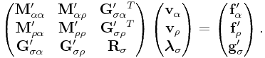
The identity submatrices make it easy to solve for ![]() and
and ![]() :
:
and hence reduce the system to
 |
(0.20) |
where
| (0.21) | ||||
| (0.22) | ||||
| (0.23) | ||||
| (0.24) |
If ![]() , then the above calculations simplify to
, then the above calculations simplify to ![]() and
and ![]() . To see that this is generally the
case, we note that typically
. To see that this is generally the
case, we note that typically ![]() . If
. If ![]() is
constant, then
is
constant, then ![]() . Otherwise, when
. Otherwise, when ![]() is not constant (as
happens in the case of point-frame attachments), we can replace
is not constant (as
happens in the case of point-frame attachments), we can replace ![]() in the main calculation with
in the main calculation with ![]() , and so continue to
allow
, and so continue to
allow ![]() .
.
The null-space reduction can be accomplished using the matrix operation
 |
where
 |
Moreover, this can be achieved on an attachment-by-attachment basis
using a series of operations ![]() , where
, where
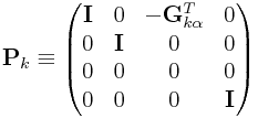 |
is the reduction matrix for a particular attachment. It is possible to
show that for two attachments ![]() and
and ![]() ,
, ![]() and
so the order of operations does not matter.
and
so the order of operations does not matter.
0.18 Attaching to an attached component
The analysis of the previous section assumed that attachments are always made to components which are not themselves attached. If this is not the case, then (0.18) is replaced by
and so the identity matrices in (0.19) no longer
appear. However, if there are no loops in the attachment relationships
(i.e., the attachment structure forms a directed acyclic graph), then
the null-space reduction can still be done, one attachment at a time,
starting with those to which no other components are attached. To see
this, let the attached system be partitioned into active components
![]() , the single component
, the single component ![]() to which no other components are
attached, and the remaining attached components
to which no other components are
attached, and the remaining attached components ![]() . This leads to
the system
. This leads to
the system
 |
(0.25) |
which can be reduced to
 |
(0.26) |
where
| (0.27) | ||||
| (0.28) | ||||
| (0.29) | ||||
| (0.30) | ||||
| (0.31) | ||||
| (0.32) | ||||
| (0.33) | ||||
| (0.34) | ||||
| (0.35) |
As mentioned above, we can often assume that ![]() .
.
Now, assuming that the attachments form a directed acyclic graph,
order this graph such that for each attached component ![]() , its masters are
either unattached or attached only to components
, its masters are
either unattached or attached only to components ![]() . If
attachments are then eliminated in this order, we can be assured that
each attached component
. If
attachments are then eliminated in this order, we can be assured that
each attached component ![]() is not itself attached to by any of the remaining
attachments, and so (0.26) can again be
placed in the form (0.25) and the
elimination can proceed recursively.
is not itself attached to by any of the remaining
attachments, and so (0.26) can again be
placed in the form (0.25) and the
elimination can proceed recursively.
If we wish to compute only the forces imparted by the attached
components, we can recursively compute ![]() and
and ![]() in the
prescribed order.
in the
prescribed order.
Velocities of the attached components can be determined by traversing the attachments in reverse order, using the formula
where ![]() only contains entries for components
only contains entries for components ![]() and hence
the velocities
and hence
the velocities ![]() have already been updated.
have already been updated.
One important thing to note from (0.35) is that if a
component is attached to more than one master, the resulting mass
matrix for those masters is no longer block diagonal. For
example, if we have a particle of mass ![]() attached to two
particles with masses
attached to two
particles with masses ![]() and
and ![]() , respectively, via
the formula
, respectively, via
the formula
then the mass matrix for particles 1 and 2 is transformed from
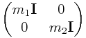 |
into
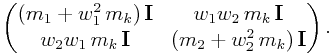 |
0.19 Adjustments to mass and fictitous forces arising from attachments
When a component ![]() is attached to a master, equations
(0.21) and (0.23) adjust the
master’s mass and force (including fictitous forces) to account for
the attached component’s mass. We will demonstrate this here
for the case of a particle with mass
is attached to a master, equations
(0.21) and (0.23) adjust the
master’s mass and force (including fictitous forces) to account for
the attached component’s mass. We will demonstrate this here
for the case of a particle with mass ![]() attached to a rigid body at a
location
attached to a rigid body at a
location ![]() with respect to the body frame’s origin.
with respect to the body frame’s origin.
Let ![]() be the particle’s velocity in world coordinates,
be the particle’s velocity in world coordinates,
![]() be the body’s spatial velocity in rotated body
coordinates, and
be the body’s spatial velocity in rotated body
coordinates, and ![]() be the rotation transform from
body to world coordinates. The attachment constraint
then takes the form
be the rotation transform from
body to world coordinates. The attachment constraint
then takes the form
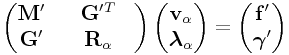
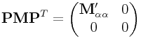
| (0.36) |
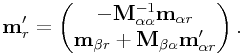
so that, with respect to (0.19),
The change in the effective inertia ![]() of the body can then be calculated from
(0.21) with
of the body can then be calculated from
(0.21) with ![]() :
:
![{\bf M}^{{\prime}}={\bf M}+m\,{\bf G}_{{\beta\alpha}}^{T}{\bf G}_{{\beta\alpha}}={\bf M}+\left(\begin{matrix}m{\bf I}&-m\,[{\bf c}]\\
m\,[{\bf c}]&-m\,[{\bf c}][{\bf c}]\end{matrix}\right),](mi/mi289.png) |
which corresponds to adding the inertia of a point pass located at ![]() with
respect to the body’s frame.
Applying the Newton-Euler equations to this point inertia,
we obtain
with
respect to the body’s frame.
Applying the Newton-Euler equations to this point inertia,
we obtain
![\left(\begin{matrix}m{\bf I}&-m\,[{\bf c}]\\
m\,[{\bf c}]&-m\,[{\bf c}][{\bf c}]\end{matrix}\right)\left(\begin{matrix}{\bf a}\\
\dot{\boldsymbol{\omega}}\end{matrix}\right)=\left(\begin{matrix}{\bf f}\\
\boldsymbol{\tau}\end{matrix}\right)+\left(\begin{matrix}-m\,\boldsymbol{\omega}\times\boldsymbol{\omega}\times{\bf c}\\
m\,\boldsymbol{\omega}\times{\bf c}\times{\bf c}\times\boldsymbol{\omega}\end{matrix}\right),](mi/mi229.png) |
where ![]() is the acceleration of the body given in
rotated body coordinates (with
is the acceleration of the body given in
rotated body coordinates (with
![]() ).
We therefore expect the attachment to add the fictitous forces
given by the rightmost vector in (0.19).
).
We therefore expect the attachment to add the fictitous forces
given by the rightmost vector in (0.19).
![m\,\left(\begin{matrix}-{\bf R}_{{BW}}^{T}\\
-[{\bf c}]\,{\bf R}_{{BW}}^{T}\end{matrix}\right)\left(\begin{matrix}{\bf R}_{{BW}}\,\boldsymbol{\omega}\times\boldsymbol{\omega}\times{\bf c}\end{matrix}\right)=\left(\begin{matrix}-m\,\boldsymbol{\omega}\times\boldsymbol{\omega}\times{\bf c}\\
m\,\boldsymbol{\omega}\times{\bf c}\times{\bf c}\times\boldsymbol{\omega}\end{matrix}\right),](mi/mi260.png)
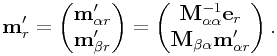
0.20 Attachments for one-dimensional constraints
Suppose we have a one-dimensional constraint, so that ![]() is
is ![]() . Then after attachment resolution,
. Then after attachment resolution, ![]() in (0.24) will be sparse, except for a number
of row vectors
in (0.24) will be sparse, except for a number
of row vectors ![]() ,
, ![]() , which are
, which are ![]() , with
, with
![]() the velocity size of component
the velocity size of component ![]() .
.
Now, if we want to apply the constraint ![]() in isolation to project
a velocity, we have
in isolation to project
a velocity, we have
which turns into
 |
Each term ![]() is the effective inverse inertia
in the direction implied by
is the effective inverse inertia
in the direction implied by ![]() .
.
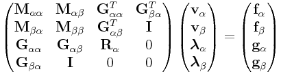
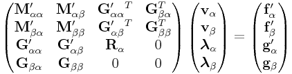
0.21 Reduction of KKT system with parametrically controlled variables
In this section we consider a system in which a set of components ![]() is controlled parametrically. Partitioning this system between
is controlled parametrically. Partitioning this system between
![]() , the active components
, the active components ![]() , and the attached components
, and the attached components
![]() , and letting
, and letting ![]() denote the union of the active and
parametrically controlled components, we obtain
denote the union of the active and
parametrically controlled components, we obtain
 |
By eliminating the attachments, we arrive at
 |
where
Since ![]() is given, we can solve for
is given, we can solve for ![]() as
as
and reduce the rest of the system to
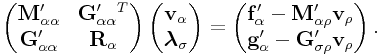 |
0.22 Jacobians for Frame Springs
A frame spring provides elastic restoring forces based on the
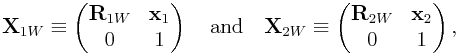
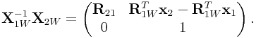
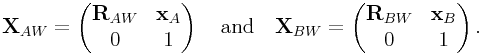
difference in position and orientation between two frames ![]() and
and ![]() (see Figure 0.2). If these frames
are described with respect to world coordinates by
(see Figure 0.2). If these frames
are described with respect to world coordinates by ![]() and
and ![]() ,
with
,
with
 |
then the displacement between the two is given by
 |
Here ![]() is the rotational transformation from
frame
is the rotational transformation from
frame ![]() to frame
to frame ![]() ; in the discussion below,
; in the discussion below, ![]() will in
general denote a rotation from frame
will in
general denote a rotation from frame ![]() to frame
to frame ![]() .
.
If ![]() and
and ![]() are the
rotation axis and angle associated with
are the
rotation axis and angle associated with ![]() , and
, and ![]() and
and
![]() are translational and rotational stiffnesses, then the
restoring forces and torques felt respectively in frames
are translational and rotational stiffnesses, then the
restoring forces and torques felt respectively in frames ![]() and
and
![]() are given by
are given by
| (0.37) |
In addition, if ![]() and
and ![]() are the angular velocities of
frames
are the angular velocities of
frames ![]() and
and ![]() (expressed in world coordinates), we can also
define damping forces according to
(expressed in world coordinates), we can also
define damping forces according to
| (0.38) |
In practice, frames ![]() and
and ![]() are rigidly connected to a secondary
pair of frames
are rigidly connected to a secondary
pair of frames ![]() and
and ![]() , whose transformations to world coordinates
are given by
, whose transformations to world coordinates
are given by
 |
Frames ![]() and
and ![]() are typically the coordinate frames of rigid bodies
and are the entities associated with dynamic calculations,
and so we need to determine forces and Jacobians with
respect to these. The rigid transformations from
are typically the coordinate frames of rigid bodies
and are the entities associated with dynamic calculations,
and so we need to determine forces and Jacobians with
respect to these. The rigid transformations from ![]() and
and ![]() to
to ![]() and
and ![]() are given by
are given by ![]() and
and ![]() , where
, where
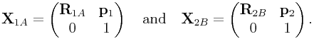 |
Mapping (0.37) and (0.38) into ![]() and
and ![]() yields
yields
| (0.39) |
and
| (0.40) |
If ![]() ,
, ![]() ,
, ![]() and
and ![]() are the translational and
rotational velocities of
are the translational and
rotational velocities of ![]() and
and ![]() (in world coordinates),
and
(in world coordinates),
and ![]() and
and ![]() are the world coordinate representations of
are the world coordinate representations of ![]() and
and ![]() ,
the the translational velocities
,
the the translational velocities ![]() and
and ![]() are described by
are described by
| (0.41) |
while the rotational velocities satisfy
| (0.42) |
0.22.1 Position Jacobian
In this section we develop the position Jacobian, which describes the
variations in forces arising from variations ![]() ,
,
![]() ,
, ![]() , and
, and ![]() in the position and
orientation of
in the position and
orientation of ![]() and
and ![]() . These will nominally be given in the
coordinates of the associated frame; otherwise, the coordinate frame
will be indicated. Conversion of these quantities between frames is
given by an appropriate rotational transform:
. These will nominally be given in the
coordinates of the associated frame; otherwise, the coordinate frame
will be indicated. Conversion of these quantities between frames is
given by an appropriate rotational transform: ![]() ,
, ![]() , etc.
, etc.
We begin with frame ![]() and the stiffness force
and the stiffness force ![]() described by (0.39).
Because of the rigid coupling between
described by (0.39).
Because of the rigid coupling between ![]() and
and ![]() and
and ![]() and
and
![]() , the variations of
, the variations of ![]() and
and ![]() depend on both
the translational and rotational variations in
depend on both
the translational and rotational variations in ![]() and
and ![]() :
:
Also, since ![]() and
and ![]() are given in world coordinates, when
frame
are given in world coordinates, when
frame ![]() rotates, the resulting
rotates, the resulting ![]() will be changed by
will be changed by ![]() . With respect to
. With respect to ![]() , this variation is
described by
, this variation is
described by ![]() , where
, where ![]() . Putting all this together, we find that the
variation of
. Putting all this together, we find that the
variation of ![]() is given by
is given by
| (0.43) |
The damping force ![]() of (0.40) also varies with
position, because the velocities
of (0.40) also varies with
position, because the velocities ![]() and
and ![]() depend on
the orientations of
depend on
the orientations of ![]() and
and ![]() . Specifically, from (0.41),
we have
. Specifically, from (0.41),
we have
which varies with orientation because ![]() does. In particular,
does. In particular,
![]() , and so
, and so
Similarly,
and
Adding in the rotational term ![]() , the
positional variation in
, the
positional variation in
![]() is then
is then
| (0.44) |
To determine the variation of ![]() ,
we need to determine the variation of
,
we need to determine the variation of ![]() . This can be
done by finding
. This can be
done by finding ![]() in terms of the angular velocity
in terms of the angular velocity ![]() of frame
of frame ![]() with respect to frame
with respect to frame ![]() , as represented in frame
, as represented in frame ![]() .
We begin by finding the derivative of a quaternion
.
We begin by finding the derivative of a quaternion ![]() which gives the orientation
of
which gives the orientation
of ![]() with respect to
with respect to ![]() . Differentiating each term and equating
it with the corresponding term in (0.1) yields
. Differentiating each term and equating
it with the corresponding term in (0.1) yields
From this we obtain
and
Then:
which can be rearranged into
| (0.45) |
which matches the results obtained by Sebastian Grassia in A
Practical Parameterization of 2 and 3 Degree of Freedom Rotations.
(In that paper, ![]() is represented by a vector
is represented by a vector ![]() ,
,
![]() is given in terms of
is given in terms of ![]() instead of
instead of ![]() ,
and
,
and ![]() is specified using the rotated frame (i.e., frame
is specified using the rotated frame (i.e., frame ![]() )
instead of the base frame.) In the case
where
)
instead of the base frame.) In the case
where ![]() , we can use
, we can use
to obtain ![]() .
.
In the above analysis, ![]() and
and ![]() represent the rotation and
angular velocity of frame 2 with respect to 1, represented in frame 1,
so that
represent the rotation and
angular velocity of frame 2 with respect to 1, represented in frame 1,
so that ![]() . For variations
in orientation,
. For variations
in orientation, ![]() is replaced by
is replaced by ![]() . Noting
that
. Noting
that ![]() ,
,
![]() , and
, and ![]() , we obtain
, we obtain
| (0.46) |
In this expression there is no rotational term involving
![]() term. That is
because the derivative of
term. That is
because the derivative of ![]() expressed by
expressed by ![]() is already
with respect to the rotating frame. However, it is convenient to
incorporate a
is already
with respect to the rotating frame. However, it is convenient to
incorporate a ![]() term for consistency with other
components of the Jacobian. Letting
term for consistency with other
components of the Jacobian. Letting ![]() ,
it is easy to verify that
,
it is easy to verify that
since
| (0.47) |
differs from ![]() only in the sign of the
only in the sign of the ![]() term.
This allows us to reformulate (0.46) as
term.
This allows us to reformulate (0.46) as
| (0.48) |
The positional variation of ![]() is due only to rotational
effects and the dependence on
is due only to rotational
effects and the dependence on ![]() :
:
| (0.49) |
Turning our attention to frame ![]() , and
, and ![]() ,
, ![]() , and
, and
![]() from (0.39) and (0.40), it
is easy to show that
from (0.39) and (0.40), it
is easy to show that
| (0.50) |
and
| (0.51) |
For ![]() , we need to take the derivative of
, we need to take the derivative of ![]() :
:
where again ![]() .
Since
.
Since ![]() and
and ![]() is constant, we
have
is constant, we
have
and therefore
Replacing ![]() with
with ![]() ,
we can obtain
,
we can obtain
which we can again be rearranged to contain a
![]() term:
term:
| (0.52) |
Finally, we have
| (0.53) |
Equations (0.43), (0.44), (0.48),
(0.49),
(0.50), (0.51), (0.52) and (0.53)
can be
combined to form the positional Jacobian ![]() which satisfies
which satisfies
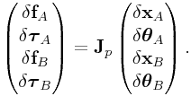 |
where we define ![]() ,
,
![]() ,
,
![]() , and
, and
![]() .
Letting
.
Letting ![]() denote the
denote the ![]() -th
-th ![]() block of
block of ![]() ,
,
![]() is then
given by
is then
given by
![\left(\begin{matrix}-k_{t}{\bf I}&k_{t}[{\bf p}_{1}]+d_{t}[\boldsymbol{\omega}_{A}][{\bf p}_{1}]+[{}^{A}{\bf f}_{1}]&k_{t}{\bf R}_{{BA}}&-k_{t}{\bf R}_{{BA}}[{\bf p}_{2}]-d_{t}{\bf R}_{{BA}}[\boldsymbol{\omega}_{B}][{\bf p}_{2}]\\
-k_{t}[{\bf p}_{1}]&[{\bf p}_{1}]{\bf J}_{{01}}-k_{r}{\bf R}_{{1A}}{\bf U}^{T}{\bf R}_{{A1}}+[{}^{A}\boldsymbol{\tau}_{1}]&k_{t}[{\bf p}_{1}]{\bf R}_{{BA}}&[{\bf p}_{1}]{\bf J}_{{03}}+k_{r}{\bf R}_{{1A}}{\bf U}{\bf R}_{{B1}}\\
k_{t}{\bf R}_{{AB}}&-k_{t}{\bf R}_{{AB}}[{\bf p}_{1}]-d_{t}{\bf R}_{{AB}}[\boldsymbol{\omega}_{A}][{\bf p}_{1}]&-k_{t}{\bf I}&k_{t}[{\bf p}_{2}]+d_{t}[\boldsymbol{\omega}_{B}][{\bf p}_{2}]+[{}^{B}{\bf f}_{2}]\\
k_{t}[{\bf p}_{2}]{\bf R}_{{AB}}&[{\bf p}_{2}]{\bf J}_{{21}}+k_{r}{\bf R}_{{1B}}{\bf U}^{T}{\bf R}_{{A1}}&-k_{t}[{\bf p}_{2}]&[{\bf p}_{2}]{\bf J}_{{23}}-k_{r}{\bf R}_{{1B}}{\bf U}{\bf R}_{{B1}}+[{}^{B}\boldsymbol{\tau}_{2}]\end{matrix}\right).](mi/mi218.png) |
The inputs and outputs for the above matrix are given with respect to
local frame coordinates, and the quantities within the matrix itself
are given with respect to either frame ![]() or
or ![]() , depending on the
sub-block.
, depending on the
sub-block.
0.22.2 Velocity Jacobian
The velocity Jacobian describes the variation in damping forces
(0.40) arising from variations ![]() ,
,
![]() ,
, ![]() , and
, and ![]() in the translational
and rotational velocities of
in the translational
and rotational velocities of ![]() and
and ![]() . Starting with
. Starting with ![]() and
and
![]() in (0.40), and using (0.41) and
(0.42), it is easy to show that
in (0.40), and using (0.41) and
(0.42), it is easy to show that
| (0.54) |
and
| (0.55) |
Likewise, for ![]() and
and ![]() , we have
, we have
| (0.56) |
and
| (0.57) |
Assembling (0.54), (0.55), (0.56)
and (0.57) yields the velocity Jacobian ![]() ,
which satisfies
,
which satisfies
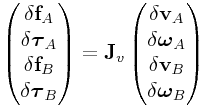 |
with ![]() given by
given by
![\left(\begin{matrix}-d_{t}{\bf I}&d_{t}[{\bf p}_{1}]&d_{t}{\bf R}_{{BA}}&-d_{t}{\bf R}_{{BA}}[{\bf p}_{2}]\\
-d_{t}[{\bf p}_{1}]&-d_{r}{\bf I}+d_{t}[{\bf p}_{1}][{\bf p}_{1}]&d_{t}[{\bf p}_{1}]{\bf R}_{{BA}}&d_{r}{\bf R}_{{BA}}-d_{t}[{\bf p}_{1}]{\bf R}_{{BA}}[{\bf p}_{2}]\\
d_{t}{\bf R}_{{AB}}&-d_{t}{\bf R}_{{AB}}[{\bf p}_{1}]&-d_{t}{\bf I}&d_{t}[{\bf p}_{2}]\\
d_{t}[{\bf p}_{2}]{\bf R}_{{AB}}&d_{r}{\bf R}_{{AB}}-d_{t}[{\bf p}_{2}]{\bf R}_{{AB}}[{\bf p}_{1}]&-d_{t}[{\bf p}_{2}]&-d_{r}{\bf I}+d_{t}[{\bf p}_{2}][{\bf p}_{2}]\\
\end{matrix}\right).](mi/mi217.png) |
0.22.3 Jacobians in world coordinates
The Jacobians derived in the previous two sections are each expressed with respect to body coordinates. In cases where the body velocities are expressed in world coordinates, the Jacobians must be adjusted to reflect this.
Beginning with the velocity Jacobian, the corresponding matrix
![]() in which inputs and outputs are given with world
coordinates is obtained from
in which inputs and outputs are given with world
coordinates is obtained from
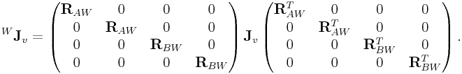 |
(0.58) |
Making use of the identity
where ![]() is a rotation, we then obtain
is a rotation, we then obtain
![{}^{W}{\bf J}_{v}=\left(\begin{matrix}-d_{t}{\bf I}&d_{t}[{\bf p}_{1}]&d_{t}{\bf I}&-d_{t}[{\bf p}_{2}]\\
-d_{t}[{\bf p}_{1}]&-d_{r}{\bf I}+d_{t}[{\bf p}_{1}][{\bf p}_{1}]&d_{t}[{\bf p}_{1}]&d_{r}{\bf I}-d_{t}[{\bf p}_{1}][{\bf p}_{2}]\\
d_{t}{\bf I}&-d_{t}[{\bf p}_{1}]&-d_{t}{\bf I}&d_{t}[{\bf p}_{2}]\\
d_{t}[{\bf p}_{2}]&d_{r}{\bf I}-d_{t}[{\bf p}_{2}][{\bf p}_{1}]&-d_{t}[{\bf p}_{2}]&-d_{r}{\bf I}+d_{t}[{\bf p}_{2}][{\bf p}_{2}]\\
\end{matrix}\right),](mi/mi410.png) |
with all quantities expressed in world coordinates.
Applying the same formulation to the position Jacobian ![]() yields
the result
yields
the result
![\left(\begin{matrix}-k_{t}{\bf I}&k_{t}[{\bf p}_{1}]+d_{t}[\boldsymbol{\omega}_{A}][{\bf p}_{1}]+[{}^{W}{\bf f}_{1}]&k_{t}{\bf I}&-k_{t}[{\bf p}_{2}]-d_{t}[\boldsymbol{\omega}_{B}][{\bf p}_{2}]\\
-k_{t}[{\bf p}_{1}]&[{\bf p}_{1}]{\bf J}_{{01}}-k_{r}{}^{W}{\bf U}^{T}+[{}^{W}\boldsymbol{\tau}_{1}]&k_{t}[{\bf p}_{1}]&[{\bf p}_{1}]{\bf J}_{{03}}+k_{r}{}^{W}{\bf U}\\
k_{t}{\bf I}&-k_{t}[{\bf p}_{1}]-d_{t}[\boldsymbol{\omega}_{A}][{\bf p}_{1}]&-k_{t}{\bf I}&k_{t}[{\bf p}_{2}]+d_{t}[\boldsymbol{\omega}_{B}][{\bf p}_{2}]+[{}^{W}{\bf f}_{2}]\\
k_{t}[{\bf p}_{2}]&[{\bf p}_{2}]{\bf J}_{{21}}+k_{r}{}^{W}{\bf U}^{T}&-k_{t}[{\bf p}_{2}]&[{\bf p}_{2}]{\bf J}_{{23}}-k_{r}{}^{W}{\bf U}+[{}^{W}\boldsymbol{\tau}_{2}]\end{matrix}\right),](mi/mi219.png) |
(0.59) |
again with all quantities expressed in world coordinates
and ![]() defined by (0.45)
with
defined by (0.45)
with ![]() expressed in world coordinates.
However, because of rotating coordinate frames, this is not
the world coordinate Jacobian. Consider first
expressed in world coordinates.
However, because of rotating coordinate frames, this is not
the world coordinate Jacobian. Consider first ![]() . Differentiation yields
. Differentiation yields
where we have used (0.37) and (0.39)
to determine that ![]() .
This eliminates the
.
This eliminates the ![]() term in the
term in the ![]() block
of (0.59), while a similar derivation eliminates the
block
of (0.59), while a similar derivation eliminates the
![]() term in the
term in the ![]() block.
Next, from (0.37) and (0.39)
we can determine that
block.
Next, from (0.37) and (0.39)
we can determine that
and therefore
This eliminates the ![]() term from the
term from the ![]() block in
(0.59) and adds a
block in
(0.59) and adds a ![]() term in its
place. A similar derivation eliminates the
term in its
place. A similar derivation eliminates the
![]() term in the
term in the ![]() block and adds
block and adds ![]() .
Together, these adjustments lead us to the position Jacobian in world coordinates:
.
Together, these adjustments lead us to the position Jacobian in world coordinates:
![{}^{W}{\bf J}_{p}=\left(\begin{matrix}-k_{t}{\bf I}&k_{t}[{\bf p}_{1}]+d_{t}[\boldsymbol{\omega}_{A}][{\bf p}_{1}]&k_{t}{\bf I}&-k_{t}[{\bf p}_{2}]-d_{t}[\boldsymbol{\omega}_{B}][{\bf p}_{2}]\\
-k_{t}[{\bf p}_{1}]&[{\bf p}_{1}]{\bf J}_{{01}}-k_{r}{}^{W}{\bf U}^{T}+[{}^{W}{\bf f}_{1}][{\bf p}_{1}]&k_{t}[{\bf p}_{1}]&[{\bf p}_{1}]{\bf J}_{{03}}+k_{r}{}^{W}{\bf U}\\
k_{t}{\bf I}&-k_{t}[{\bf p}_{1}]-d_{t}[\boldsymbol{\omega}_{A}][{\bf p}_{1}]&-k_{t}{\bf I}&k_{t}[{\bf p}_{2}]+d_{t}[\boldsymbol{\omega}_{B}][{\bf p}_{2}]\\
k_{t}[{\bf p}_{2}]&[{\bf p}_{2}]{\bf J}_{{21}}+k_{r}{}^{W}{\bf U}^{T}&-k_{t}[{\bf p}_{2}]&[{\bf p}_{2}]{\bf J}_{{23}}-k_{r}{}^{W}{\bf U}+[{}^{W}{\bf f}_{2}][{\bf p}_{2}]\end{matrix}\right).](mi/mi409.png) |
0.23 Non-symmetry of Jacobians for Rigid Body Forces
Consider a rigid body with a constant force (in world coordinates)
![]() acting on its center of mass. The force in body coordinates
is given by
acting on its center of mass. The force in body coordinates
is given by
If ![]() is a variation in
the body’s orientation, then the resulting variation
is a variation in
the body’s orientation, then the resulting variation ![]() is given by
is given by
from which we can deduce that
![\frac{\partial{}^{B}{\bf f}}{\partial\boldsymbol{\theta}}=[{\bf R}_{{WB}}{}^{W}{\bf f}]](mi/mi206.png) |
which is asymmetrical.
Moreover, this asymmetry cannot be averted by formulating the equations of motion in world coordinates instead of body coordinates, because then the inertia matrix varies with orientation in a way that is also asymmetrical.
To see this, consider an inertia matrix located at the body’s center of mass. In world coordinates, this is
 |
The variation ![]() in response to
in response to ![]() is then
is then
 |
|||
![\displaystyle=\left(\begin{matrix}0&0\\
0&[{}^{W}\boldsymbol{\omega}]{}^{W}{\bf J}-{}^{W}{\bf J}[{}^{W}\boldsymbol{\omega}]\end{matrix}\right)](mi/mi27.png) |
where
Now consider the implicit integration formula:
Since ![]() , we have
, we have
Multiplying the implicit formula through by ![]() yeilds
yeilds
Expanding the ![]() term, we obtain
term, we obtain
![\displaystyle=\left(\begin{matrix}0&0\\
0&[{}^{W}\boldsymbol{\omega}]{}^{W}{\bf J}-{}^{W}{\bf J}[{}^{W}\boldsymbol{\omega}]\end{matrix}\right)\left(\begin{matrix}1/m{\bf I}&0\\
0&{}^{W}{\bf J}^{{-1}}\end{matrix}\right)\left(\begin{matrix}{\bf f}_{t}\\
\boldsymbol{\tau}\end{matrix}\right)](mi/mi28.png) |
|||
![\displaystyle=\left(\begin{matrix}0\\
([{}^{W}\boldsymbol{\omega}]{}^{W}{\bf J}-{}^{W}{\bf J}[{}^{W}\boldsymbol{\omega}]){}^{W}{\bf J}^{{-1}}\boldsymbol{\tau}\end{matrix}\right)](mi/mi30.png) |
where ![]() and
and ![]() are the translational force and torque.
The lower term can be formulated as
are the translational force and torque.
The lower term can be formulated as ![]() ,
where
,
where
is clearly assymmetric.