1.2 Simulation overview
An overview of the ArtiSynth simulation mechanism is given here. More details are given in [11] and in the related overview paper.
1.2.1 Model advancement
ArtiSynth simulation works by advancing models forward in time using a series of time steps, with a physics integrator updating positions, velocities and forces for all of the dynamic components over each step. The step size is usually fixed, but can vary between models and also over different time ranges, as described in more detail in the “Advancing Models in Time” section of the ArtiSynth Reference Manual.
Simulation happens under the control of a scheduler, which determines the next time to advance to and then advances the root model using its advance() method. In pseudo-code, this looks like:
Most often, the next advance time is determined by adding the value of the root model’s maxStepSize property to t0.
Within its advance() method, the root model in turn calls the advance() methods for its collection of models, while also calling the apply() methods for the model agents. For each model, the advancement sequence typically looks like that shown in Figure 1.1, with any input probes and controllers called before the advance() method and any monitors and output probes called after. The preadvance() method is an additional method that a model can use to perform pre-step initialization before input probes and controllers are called.
By default, the update interval ![]() in Figure 1.1 equals
the maxStepSize of the root model. However,
in Figure 1.1 equals
the maxStepSize of the root model. However, ![]() will be less if required
by the model’s own maxStepSize value, or a smaller (explicit) update
interval for any of the output probes. Figure 1.1 also
assumes that all of the model agents are explicitly associated with the
model. Input probes and controllers that are not associated with the
model will be applied before the preadvance() method, and monitors
and output probes not associated with the model will be called after those that
are. Again, more precise details on this are given in the “Advancing Models in
Time” section of the
ArtiSynth Reference Manual.
will be less if required
by the model’s own maxStepSize value, or a smaller (explicit) update
interval for any of the output probes. Figure 1.1 also
assumes that all of the model agents are explicitly associated with the
model. Input probes and controllers that are not associated with the
model will be applied before the preadvance() method, and monitors
and output probes not associated with the model will be called after those that
are. Again, more precise details on this are given in the “Advancing Models in
Time” section of the
ArtiSynth Reference Manual.
1.2.2 Full coordinate formulation
It is important to understand that ArtiSynth uses a full coordinate
formulation, in which the position and velocity of each dynamic body is both
represented and solved using full, or unconstrained, coordinates, with extra
equations added to the system solve to account for constraints such as joints
and contact. In particular, point positions and velocities are represented
using 3-vectors, while the “positions” of RigidBody and Frame
components are represented as the translation and orientation of their
coordinate frames. Internally, these frames are stored as a 3-vector plus a
quaternion, but they are most often presented to the application as the body’s
pose, which is the ![]() homogeneous transformation
homogeneous transformation ![]() that
maps points from body to world coordinates:
that
maps points from body to world coordinates:
Here ![]() is a
is a ![]() rotation matrix and
rotation matrix and ![]() is a 3-vector
giving the location of the frame origin in world coordinates. The “velocity”
of RigidBody and Frame components is the spatial velocity
is a 3-vector
giving the location of the frame origin in world coordinates. The “velocity”
of RigidBody and Frame components is the spatial velocity
where ![]() and
and ![]() give the coordinate frame’s translational and
angular velocity in world coordinates. See Sections A.2
and A.5 for more details.
give the coordinate frame’s translational and
angular velocity in world coordinates. See Sections A.2
and A.5 for more details.
In contrast, some other simulation systems, including OpenSim [7], use reduced coordinates, in which the system dynamics are formulated using a smaller set of coordinates (such as joint angles) that implicitly take the system’s constraints into account. For example, a two degree-of-freedom (DOF) double pendulum in ArtiSynth is described using 12 degrees of freedom (six for each of the two bodies), with 10 constraint equations added to reduce the net DOF to two, while in OpenSim, a double pendulum would be described using only its two joint angles.
Each methodology has its own advantages. Reduced formulations yield systems with fewer degrees of freedom and no constraint errors. On the other hand, full coordinates make it easier to combine and connect a wide range of components, including rigid bodies and FE models, and they also allow modeling of situations where constraints are compliant (i.e., soft) such that the bodies connected to them can assume arbitrary poses with respect to each other. The speed advantages of reduced coordinates are much less important in ArtiSynth, where the main performance bottleneck is usually the computational requirements of FE models.
1.2.3 Time stepping and integration physics
This section describes the mechanical simulation that takes place inside the
advance() method of MechModel. An integrator is used to advance the
model from time ![]() to time
to time ![]() , corresponding to a time step given by
, corresponding to a time step given by
![]() . Several integrators are available and may be selected via
the model’s integrator property. The ones discussed here are the
first order explicit integrator ConstrainedForwardEuler and
the first-order implicit integrator ConstrainedBackwardEuler (which
is the system default).
. Several integrators are available and may be selected via
the model’s integrator property. The ones discussed here are the
first order explicit integrator ConstrainedForwardEuler and
the first-order implicit integrator ConstrainedBackwardEuler (which
is the system default).
Let the positions, velocities, and forces associated with all the dynamic
components be denoted by the composite vectors ![]() ,
, ![]() , and
, and ![]() . In
addition, let the composite mass matrix be given by
. In
addition, let the composite mass matrix be given by ![]() . Newton’s second law
then gives
. Newton’s second law
then gives
| (1.1) |
where the ![]() term accounts for various “fictitious” forces.
term accounts for various “fictitious” forces.
Each integration step involves solving for
the velocities ![]() at time step
at time step ![]() given the velocities and forces
at step
given the velocities and forces
at step ![]() . One way to do this is to solve the expression
. One way to do this is to solve the expression
| (1.2) |
for ![]() , where
, where ![]() is the step size and
is the step size and
![]() . Given the updated velocities
. Given the updated velocities ![]() , one can
determine
, one can
determine ![]() from
from
| (1.3) |
where ![]() accounts for situations (such as rigid bodies) where
accounts for situations (such as rigid bodies) where
![]() , and then solve for the updated positions using
, and then solve for the updated positions using
| (1.4) |
(1.2) and (1.4) by themselves comprise a simple symplectic Euler integrator.
In addition to forces, bilateral and unilateral constraints give rise to (generally) nonlinear constraint equations of the form
| (1.5) |
Bilateral constraints are equality constraints that may include rigid body
joints, FEM incompressibility, and point-surface constraints, while unilateral
constraints are inequality constraints that include contact forces, friction
and joint limits. Linearizing (1.5) leads to locally linear
constraints on the velocity ![]() of the form
of the form
| (1.6) |
where ![]() and
and ![]() are the derivative matrices of
are the derivative matrices of ![]() . Because
. Because ![]() and
and
![]() are evaluated at step
are evaluated at step ![]() but generally vary in time, we can use their
time derivatives to improve constraint satisfaction for
but generally vary in time, we can use their
time derivatives to improve constraint satisfaction for ![]() by modifying
(1.6) to
by modifying
(1.6) to
| (1.7) |
where
| (1.8) |
Constraints give rise to constraint forces (in the directions ![]() and
and
![]() ) which supplement the forces of (1.1) in order to
enforce the constraint conditions. In addition, for unilateral constraints, we
have a complementarity condition in which
) which supplement the forces of (1.1) in order to
enforce the constraint conditions. In addition, for unilateral constraints, we
have a complementarity condition in which ![]() implies no constraint
force, and a constraint force implies
implies no constraint
force, and a constraint force implies ![]() . Any given constraint
usually involves only a few dynamic components and so
. Any given constraint
usually involves only a few dynamic components and so ![]() and
and ![]() are
generally sparse.
are
generally sparse.
Adding constraints to the velocity solve (1.2) leads to a mixed linear complementarity problem (MLCP) of the form
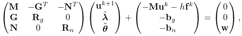 |
|||
| (1.9) |
where ![]() is a slack variable,
is a slack variable, ![]() and
and ![]() give the
constraint force impulses over the time step, and the constraint offsets
give the
constraint force impulses over the time step, and the constraint offsets ![]() and
and ![]() are typically set to
are typically set to ![]() and
and ![]() as per
(1.8).
as per
(1.8). ![]() and
and ![]() are optional diagonal regularization terms, which if non-zero serve to soften the constraints,
either to handle redundancy or to simulate physical compliance, as discussed
later in Sections 3.4.9
and 8.6.1. If
are optional diagonal regularization terms, which if non-zero serve to soften the constraints,
either to handle redundancy or to simulate physical compliance, as discussed
later in Sections 3.4.9
and 8.6.1. If ![]() or
or ![]() , then
, then ![]() or
or ![]() will typically also include a term related to the constraint error.
will typically also include a term related to the constraint error.
The actual constraint forces ![]() and
and ![]() can be determined by dividing
the constraint impulses by the time step
can be determined by dividing
the constraint impulses by the time step ![]() :
:
| (1.10) |
By itself, the MLCP (1.9) implements a constrained forward Euler integrator corresponding to setting the MechModel’s integrator property to ConstrainedForwardEuler.
For stiff systems, which often arise with systems containing FE models,
explicit integrators can be unstable unless the step size ![]() is set to a very
small value. This can typically be corrected by using an implicit
integrator. A first order example of this is a backward Euler integrator
in which
is set to a very
small value. This can typically be corrected by using an implicit
integrator. A first order example of this is a backward Euler integrator
in which ![]() is replaced with an approximation of
is replaced with an approximation of ![]() given by the
Taylor series expansion
given by the
Taylor series expansion
| (1.11) |
where ![]() and
and ![]() are the
negatives of the system stiffness and damping matrices,
respectively. Since
are the
negatives of the system stiffness and damping matrices,
respectively. Since
(1.11) can be reformulated as
| (1.12) |
which leads to the modified MLCP
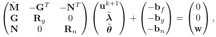 |
|||
| (1.13) |
where
The MLCP (1.13) corresponds to the default ArtiSynth integrator ConstrainedBackwardEuler. Higher order integrators, such as Newmark methods, often give rise to MLCPs with an equivalent form. Most ArtiSynth integrators use some variation of (1.13) to determine the system velocity at each time step; a description of the second order Trapezoidal integrator is given in [11].
To assemble (1.13), the MechModel component hierarchy is
traversed and the methods of the different component types are queried for the
required values. Dynamic components (type DynamicComponent) provide
![]() ,
, ![]() , and
, and ![]() ; force effectors (ForceEffector) determine
; force effectors (ForceEffector) determine ![]() and the stiffness/damping augmentation used to produce
and the stiffness/damping augmentation used to produce ![]() ; and constrainers
(Constrainer) supply
; and constrainers
(Constrainer) supply ![]() ,
, ![]() ,
, ![]() and
and ![]() .
.
1.2.4 Parametric and attached dynamic components
By default, a dynamic component is advanced through time in response to the forces applied to it. However, it is also possible to set a dynamic component to be parametric, such that it does not respond to forces and its position and/or velocity is either fixed or specified directly by the simulation. This is done by setting the component’s dynamic property to false, either through the GUI (by selecting the component(s) and choosing Edit properties ... from the context menu), or in code using the methods
| void setDynamic (boolean enable) |
Sets the dynamic property. |
| boolean isDynamic() |
Queries the dynamic property. |
Usage of setDynamic() is usually restricted to dynamic components that have mass, which include Particle and RigidBody but not Point or Frame.
Because the positions and velocities of parametric components are given, the MLCP (1.13) needs to be modified to reflect this. This involves partitioning the system velocity and force vectors into
where ![]() and
and ![]() denote the active (non-parametric) and parametric
components, respectively. The MLCP is then likewise partitioned. Considering
for simplicity the case with only bilateral constraints, this takes the form
denote the active (non-parametric) and parametric
components, respectively. The MLCP is then likewise partitioned. Considering
for simplicity the case with only bilateral constraints, this takes the form
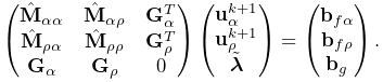 |
Since ![]() is given, the system can be reduced to
is given, the system can be reduced to
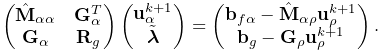 |
ArtiSynth also provides an attachment mechanism that allows dynamic components to be directly attached to other dynamic components. This is one of the primary means by which different parts of a model are connected together: points and particles (including FE nodes) can be attached to rigid bodies or other particles, and Frame components can be attached to other rigid bodies or connected to the nodes of an FE model.
When a dynamic component is attached, its position becomes a direct function of
the positions of the one or more master components to which it is
attached. For example, if a component ![]() is attached to a master component
is attached to a master component
![]() , then its position
, then its position ![]() is a function of the position
is a function of the position ![]() of
of ![]() :
:
Differentiating this yields a linear relationship between the velocities ![]() and
and ![]() of
of ![]() and
and ![]() ,
,
| (1.14) |
where ![]() is the derivative of
is the derivative of ![]() .
.
Attachments can be considered as constraints in which the positions/velocities of the attached components are constrained to be functions of the positions/velocities of the master components. While enforcement could be effected by adding velocity constraints of the form (1.14) to the system MLCP (1.13), in practice ArtiSynth actually uses the velocity constraints to preprocess the MLCP and remove the attached components from the system solve, which generally improves solve times. The attached positions/velocities are then updated after the solve based on the master positions/velocities.
As mentioned in Section 1.1.1, attachments are implemented by components which implement DynamicAttachment. These may be added to the model hierarchy separately, or, in the case of Marker and AttachedFrame components, embedded within specialized Point and Frame subclasses which are always attached.
Overall, a dynamic component can be in one of three states:
- active
-
Component is dynamic and unattached. The method isActive() returns true. The component will move in response to forces.
- parametric
-
Component is not dynamic, and is unattached. The method isParametric() returns true. The component will either remain fixed, or will move around in response to external inputs specifying the component’s position and/or velocity. One way to supply such inputs is to use controllers or input probes, as described in Section 5.
- attached
-
Component is attached. The method isAttached() returns true, and the method getAttachment() will return the actual attachment component. The component will move so as to follow the other master component(s) to which it is attached.
![[LOGO]](data:image/png;base64,iVBORw0KGgoAAAANSUhEUgAAAAsAAAAOCAYAAAD5YeaVAAAAAXNSR0IArs4c6QAAAAZiS0dEAP8A/wD/oL2nkwAAAAlwSFlzAAALEwAACxMBAJqcGAAAAAd0SU1FB9wKExQZLWTEaOUAAAAddEVYdENvbW1lbnQAQ3JlYXRlZCB3aXRoIFRoZSBHSU1Q72QlbgAAAdpJREFUKM9tkL+L2nAARz9fPZNCKFapUn8kyI0e4iRHSR1Kb8ng0lJw6FYHFwv2LwhOpcWxTjeUunYqOmqd6hEoRDhtDWdA8ApRYsSUCDHNt5ul13vz4w0vWCgUnnEc975arX6ORqN3VqtVZbfbTQC4uEHANM3jSqXymFI6yWazP2KxWAXAL9zCUa1Wy2tXVxheKA9YNoR8Pt+aTqe4FVVVvz05O6MBhqUIBGk8Hn8HAOVy+T+XLJfLS4ZhTiRJgqIoVBRFIoric47jPnmeB1mW/9rr9ZpSSn3Lsmir1fJZlqWlUonKsvwWwD8ymc/nXwVBeLjf7xEKhdBut9Hr9WgmkyGEkJwsy5eHG5vN5g0AKIoCAEgkEkin0wQAfN9/cXPdheu6P33fBwB4ngcAcByHJpPJl+fn54mD3Gg0NrquXxeLRQAAwzAYj8cwTZPwPH9/sVg8PXweDAauqqr2cDjEer1GJBLBZDJBs9mE4zjwfZ85lAGg2+06hmGgXq+j3+/DsixYlgVN03a9Xu8jgCNCyIegIAgx13Vfd7vdu+FweG8YRkjXdWy329+dTgeSJD3ieZ7RNO0VAXAPwDEAO5VKndi2fWrb9jWl9Esul6PZbDY9Go1OZ7PZ9z/lyuD3OozU2wAAAABJRU5ErkJggg==)