Finite Element Models
July 17, 2024
Contents
-
1 Finite Element Models
- 1.1 Overview
- 1.2 FEM model creation
- 1.3 FEM Geometry
-
1.4 Connecting FEM models to other components
- 1.4.1 Connecting nodes to rigid bodies or particles
- 1.4.2 Example: connecting a beam to a block
- 1.4.3 Connecting nodes directly to elements
- 1.4.4 Example: connecting two FEMs together
- 1.4.5 Finding which nodes to attach
- 1.4.6 Selecting nodes in the viewer
- 1.4.7 Example: two bodies connected by an FEM “spring”
- 1.4.8 Nodal-based attachments
- 1.4.9 Example: element vs. nodal-based attachments
- 1.5 FEM markers
- 1.6 Frame attachments
- 1.7 Incompressibility
- 1.8 Varying and augmenting material behaviors
- 1.9 Muscle activated FEM models
-
1.10 Material types
- 1.10.1 Linear
-
1.10.2 Hyperelastic materials
- 1.10.2.1 St Venant-Kirchoff material
- 1.10.2.2 Neo-Hookean material
- 1.10.2.3 Incompressible neo-Hookean material
- 1.10.2.4 Mooney-Rivlin material
- 1.10.2.5 Ogden material
- 1.10.2.6 Fung orthotropic material
- 1.10.2.7 Yeoh material
- 1.10.2.8 Arruda-Boyce material
- 1.10.2.9 Veronda-Westmann material
- 1.10.2.10 Incompressible material
- 1.10.3 Muscle materials
- 1.11 Stress, strain and strain energy
- 1.12 Rendering and Visualizations
Chapter 1 Finite Element Models
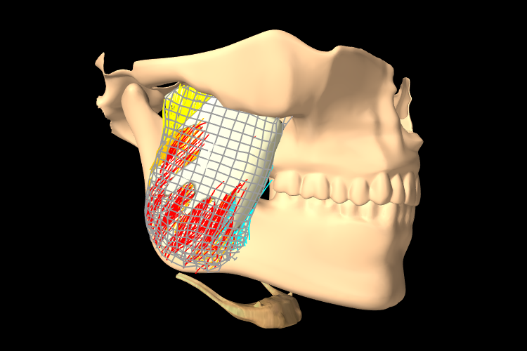
This chapter details how to construct three-dimensional finite element models, and how to couple them with the other simulation components described in previous sections (e.g. particles and rigid bodies). Finite element muscles, which have additional properties that allow them to contract given activation signals, are discussed in Section 1.9. An example FEM model of the masseter, coupled to a rigid jaw and maxilla, is shown in Figure 1.1.
1.1 Overview
The finite element method (FEM) is a numerical technique used for solving a system of partial differential equations (PDEs) over some domain. The general approach is to divide the domain into a set of building blocks, referred to as elements. These partition the space, and form local domains over which the system of equations can be locally approximated. The corners of these elements, the nodes, become control points in a discretized system. The solution is then assumed to be smoothly interpolated across the elements based on values determined at the nodes. Using this discretization, the differential system is converted into an algebraic one, which is often linearized and solved iteratively.
In ArtiSynth, the PDEs considered are the governing equations of continuum mechanics: the conservation of mass, momentum, and energy. To complete the system, a constitutive equation is required that describes the stress-strain response of the material. This constitutive equation is what distinguishes between material types. The domain is the three-dimensional space that the model occupies. This must be divided into small elements which accurately represent the geometry. Within each element, the PDEs are sampled at a set of points, referred to as integration points, and terms are numerically integrated to form an algebraic system to solve.
The purpose of the rest of this chapter is to describe the construction and use of finite elements models within ArtiSynth. It does not further discuss the mathematical framework or theory. For an in-depth coverage of the nonlinear finite element method, as applied to continuum mechanics, the reader is referred to the textbook by Bonet and Wood [bonet:fem:2000].
1.1.1 FemModel3d
The basic type of finite element model is implemented in the class FemModel3d. This class controls some properties that are used by the model as a whole. The key ones that affect simulation dynamics are:
| Property | Description |
|---|---|
| density | The density of the model |
| material | An object that describes the material’s constitutive law (i.e. its stress-strain relationship). |
| particleDamping | Proportional damping associated with the particle-like motion of the FEM nodes. |
| stiffnessDamping | Proportional damping associated with the system’s stiffness term. |
These properties can be set and retrieved using the methods
| void setDensity (double density) |
Sets the density. |
| double getDensity() |
Gets the density. |
| void setMaterial (FemMaterial mat) |
Sets the FEM’s material. |
| FemMaterial getMaterial() |
Gets the FEM’s material. |
| void setParticleDamping (double d) |
Sets the particle (mass) damping. |
| double getParticleDamping() |
Gets the particle (mass) damping. |
| void setStiffnessDamping (double d) |
Sets the stiffness damping. |
| double getStiffnessDamping() |
Gets the stiffness damping. |
Keep in mind that ArtiSynth is essentially “unitless” (Section LABEL:sec:mechii:units), so it is the responsibility of the developer to ensure that all properties are specified in a compatible way.
The density of the model is used to compute the mass distribution throughout the volume. Note that we use a diagonally lumped mass matrix (DLMM) formulation, so the mass is assumed to be concentrated at the location of the discretized FEM nodes. To allow for a spatially-varying density, densities can be explicitly set for individual elements, or masses can be explicitly set for individual nodes.
The FEM’s material property is a delegate object used to compute stress and stiffness within individual elements. It handles the constitutive component of the model, as described in more detail in Sections 1.1.3 and 1.10. In addition to the main material defined for the model, it is also possible set a material on a per-element basis, and to define additional materials which augment the behavior of the main materials (Section 1.8).
The two damping parameters are related to Rayleigh damping, which is used to dissipate energy within finite element models. There are two proportional damping terms: one related to the system’s mass, and one related to stiffness. The resulting damping force applied is
| (1.1) |
where ![]() is the value of particleDamping,
is the value of particleDamping, ![]() is the value of
stiffnessDamping,
is the value of
stiffnessDamping, ![]() is the FEM model’s lumped mass matrix,
is the FEM model’s lumped mass matrix, ![]() is
the FEM’s stiffness matrix, and
is
the FEM’s stiffness matrix, and ![]() is the concatenated vector of FEM node
velocities. Since the lumped mass matrix is diagonal, the mass-related
component of damping can be applied separately to each FEM node. Thus, the
mass component reduces to the same system as Equation (LABEL:eqn:pointdamping),
which is why it is referred to as “particle damping”.
is the concatenated vector of FEM node
velocities. Since the lumped mass matrix is diagonal, the mass-related
component of damping can be applied separately to each FEM node. Thus, the
mass component reduces to the same system as Equation (LABEL:eqn:pointdamping),
which is why it is referred to as “particle damping”.
1.1.2 Component Structure
Each FemModel3d contains several lists of subcomponents:
- nodes
-
The particle-like dynamic components of the model. These lie at the corners of the elements and carry all the mass (due to DLMM formulation).
- elements
-
The volumetric model elements. These define the 3D sub-units over which the system is numerically integrated.
- shellElements
-
The shell elements. These define additional 2D sub-units over which the system is numerically integrated.
- meshes
-
The geometry in the model. This includes the surface mesh, and any other embedded geometries.
- materials
-
Optional additional materials which can be added to the model to augment the behavior of the model’s material property. This is described in more detail in Section 1.8.
- fields
-
Optional field components which can be used to interpolate application-defined quantities over the FEM model’s domain. Fields are described in detail in Chapter LABEL:sec:fields.
The nodes, elements and meshes components are illustrated in Figure 1.2.
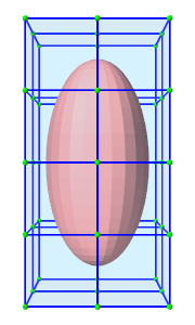 |
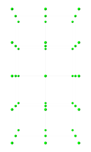 |
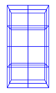 |
 |
| (a) FEM model | (b) Nodes | (c) Elements | (d) Geometry |
1.1.2.1 Nodes
The set of nodes belong to a finite element model can be obtained by the method
| PointList<FemNode3d> getNodes() |
Returns the list of FEM nodes. |
Nodes are implemented in the class FemNode3d, which is a subclass of Particle (Section LABEL:ParticlesAndSprings:sec). They are the main dynamic components of the finite element model. The key properties affecting simulation dynamics are:
| Property | Description |
|---|---|
| restPosition | The initial position of the node. |
| position | The current position of the node. |
| velocity | The current velocity of the node. |
| mass | The mass of the node. |
| dynamic | Whether the node is considered dynamic or parametric (e.g. boundary condition). |
Each of these properties has corresponding getXxx() and setXxx(...) functions to access and modify them.
The restPosition property defines the node’s position in the FEM model’s “natural” or “undeformed” state. Rest positions are used to compute an initial configuration for the model, from which strains are determined. A node’s rest position can be updated in code using the method: FemNode3d.setRestPosition(Point3d).
If any node’s rest positions are changed, the current values for stress and stiffness will become invalid. They can be manually updated using the method FemModel3d.updateStressAndStiffness() for the parent model. Otherwise, stress and stiffness will be automatically updated at the beginning of the next time step.
The properties position and velocity give the node’s current 3D state. These are common to all point-like particles, as is the mass property. Here, however, mass represents the lumped mass of the immediately surrounding material. Its value is initialized by equally dividing mass contributions from each adjacent element, given their densities. For a finer control of spatially-varying density, node masses can be set manually after FEM creation.
The FEM node’s dynamic property specifies whether or not the node is considered when computing the dynamics of the system. If not, it is treated as being parametrically controlled. This has implications when setting boundary conditions (Section 1.1.4).
1.1.2.2 Elements
Elements are the 3D volumetric spatial building blocks of the domain. Within each element, the displacement (or strain) field is interpolated from displacements at nodes:
 |
(1.2) |
where ![]() is the displacement of the
is the displacement of the ![]() th node that is adjacent to the
element, and
th node that is adjacent to the
element, and ![]() is referred to as the shape function (or
basis function) associated with that node. Elements are classified by
their shape, number of nodes, and shape function order (Table
1.1). ArtiSynth supports the following element types,
shown below with their node numberings:
is referred to as the shape function (or
basis function) associated with that node. Elements are classified by
their shape, number of nodes, and shape function order (Table
1.1). ArtiSynth supports the following element types,
shown below with their node numberings:
| TetElement | PyramidElement | WedgeElement | HexElement |
| QuadtetElement | QuadpyramidElement | QuadwedgeElement | QuadhexElement |
| Element Type | # Nodes | Order | # Integration Points |
|---|---|---|---|
| TetElement | 4 | linear | 1 |
| PyramidElement | 5 | linear | 5 |
| WedgeElement | 6 | linear | 6 |
| HexElement | 8 | linear | 8 |
| QuadtetElement | 10 | quadratic | 4 |
| QuadpyramidElement | 13 | quadratic | 5 |
| QuadwedgeElement | 15 | quadratic | 9 |
| QuadhexElement | 20 | quadratic | 14 |
The base class for all of these is FemElement3d. A numerical integration is performed within each element to create the (tangent) stiffness matrix. This integration is performed by evaluating the stress and stiffness at a set of integration points within each element, and applying numerical quadrature. The list of elements in a model can be obtained with the method
| RenderableComponentList<FemElement3d> getElements() |
Returns the list of volumetric elements. |
All objects of type FemElement3d have the following properties:
| Property | Description |
|---|---|
| density | Density of the element |
| material | An object that describes the constitutive law within the element (i.e. its stress-strain relationship). |
If left unspecified, the element’s density is inherited from the containing FemModel3d object. When set, the mass of the element is computed and divided amongst all its nodes, updating the lumped mass matrix.
1.1.2.3 Shell elements
Shell elements are additional 2D spatial building blocks which can be added to a model. They are typically used to model structures which are too thin to be easily represented by 3D volumetric elements, or to provide additional internal stiffness within a set of volumetric elements.
ArtiSynth presently supports the following shell element types, with the number of nodes, shape function order, and integration point count described in Table 1.2:
| Element Type | # Nodes | Order | # Integration Points |
|---|---|---|---|
| ShellTriElement | 3 | linear | 9 (3 if membrane) |
| ShellQuadElement | 4 | linear | 8 (4 if membrane) |
The base class for all shell elements is ShellElement3d, which contains the same density and material properties as FemElement3d, as well as the additional property defaultThickness, whose use will be described below.
The list of shell elements in a model can be obtained with the method
| RenderableComponentList<ShellElement3d> getShellElements() |
Returns the list of shell elements. |
Both the volumetric elements (FemElement3d) and the shell elements (ShellElement3d) derive from the base class FemElement3dBase. To obtain all the elements in an FEM model, both shell and volumetric, one may use the method
| ArrayList<FemElement3dBase> getAllElements() |
Returns a list of all elements. |
Each shell element can actually be instantiated in two forms:
-
•
As a regular shell element, which has a bending stiffness;
-
•
As a membrane element, which does not have bending stiffness.
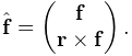
Regular shell elements are implemented using the same extensible director formulation used by FEBio [MaasFEBio2012], and more specifically the front/back node formulation [FEBioTheory2018]. Each node associated with a (regular) shell element is assigned a director, which is a 3D vector providing a normal direction and virtual thickness at that node (Figure 1.3). This virtual thickness allows us to continue to use 3D materials to provide the constitutive laws that determine the shell’s stress/strain response, including its bending behavior. It also allows us to continue to use the element’s density to determine its mass.
Director information is automatically assigned to a FemNode3d whenever one or more regular shell elements is connected to it. This information includes both the current value of the director, its rest value, and its velocity, with the difference between the first two determining the element’s bending strain. These quantities can be queried using the methods
For nodes which are not connected to regular shell elements, and therefore do not have director information assigned, these methods all return a zero-valued vector.
If not otherwise specified, the current and rest director values are
computed automatically from the surrounding (regular) shell elements,
with their value ![]() being computed from
being computed from
where ![]() is the value of the defaultThickness property and
is the value of the defaultThickness property and
![]() is the surface normal of the
is the surface normal of the ![]() -th surrounding regular shell
element.
However, if necessary, it is also possible to explicitly assign
these values, using the methods
-th surrounding regular shell
element.
However, if necessary, it is also possible to explicitly assign
these values, using the methods
ArtiSynth FEM nodes can currently support only one director, which is shared by all regular shell elements associated with that node. This effectively means that all such elements must belong to the same “surface”, and that two intersecting surfaces cannot share the same nodes.
As indicated above, shell elements can also be instantiated as membrane elements, which do not exhibit bending stiffness and therefore do not require director information. The regular/membrane distinction is specified in the element’s constructor. For example, ShellTriElement and ShellQuadElement each have constructors with the signatures:
The thickness argument specifies the defaultThickness property, while membrane determines whether or not the element is a membrane element.
While membrane elements do not require explicit director information stored at the nodes, they do make use of an inferred director that is parallel to the element’s surface normal, and has a constant length equal to the element’s defaultThickness property. This gives the element a virtual volume, which (as with regular elements) is used to determine 3D strains and to compute the element’s mass from it’s density.
1.1.2.4 Meshes
The geometry associated with a finite element model consists of a collection of meshes (e.g. PolygonalMesh, PolylineMesh, PointMesh) that move along with the model in a way that maintains the shape function interpolation equation (1.2) at each vertex location. These geometries can be used for visualizations, or for physical interactions like collisions. However, they have no physical properties themselves. FEM geometries will be discussed in more detail in Section 1.3. The list of meshes can be obtained with the method
1.1.3 Materials
The stress-strain relationship within each element is defined by a “material” delegate object, implemented by a subclass of FemMaterial. This material object is responsible for implementing the functions
which computes the stress tensor and (optionally) the tangent stiffness matrix at each integration point, based on the current local deformation at that point.
All supported materials are presented in detail in Section
1.10. The default material type is
LinearMaterial, which
linearly maps Cauchy strain ![]() onto Cauchy stress
onto Cauchy stress ![]() via
via
where ![]() is the elasticity tensor determined
from Young’s modulus and Poisson’s ratio. Anisotropic
linear materials are provided by
TransverseLinearMaterial
and
AnisotropicLinearMaterial.
Linear materials in ArtiSynth implement corotation, which removes the
rotation from the deformation gradient and allows Cauchy strain to be
applied to large
deformations [ngan:fem:2008, muller2004interactive]. Nonlinear
hyperelastic materials are also supported, including
MooneyRivlinMaterial,
OgdenMaterial,
YeohMaterial,
ArrudaBoyceMaterial,
and
VerondaWestmannMaterial.
is the elasticity tensor determined
from Young’s modulus and Poisson’s ratio. Anisotropic
linear materials are provided by
TransverseLinearMaterial
and
AnisotropicLinearMaterial.
Linear materials in ArtiSynth implement corotation, which removes the
rotation from the deformation gradient and allows Cauchy strain to be
applied to large
deformations [ngan:fem:2008, muller2004interactive]. Nonlinear
hyperelastic materials are also supported, including
MooneyRivlinMaterial,
OgdenMaterial,
YeohMaterial,
ArrudaBoyceMaterial,
and
VerondaWestmannMaterial.
1.1.4 Boundary conditions
Boundary conditions can be implemented in one of several ways:
-
1.
Explicitly setting FEM node positions/velocities
-
2.
Attaching FEM nodes to other dynamic components
-
3.
Enabling collisions
To enforce an explicit (Dirichlet) boundary condition for a set of nodes, their dynamic property must be set to false. This notifies ArtiSynth that the state of these nodes (both position and velocity) will be controlled parametrically. By disabling dynamics, a fixed boundary condition is applied. For a moving boundary, positions and velocities of the boundary nodes must be explicitly set every timestep. This can be accomplished with either a Controller (see Section LABEL:ControllersAndMonitors:sec) or an InputProbe (see Section LABEL:Probes:sec). Note that both the position and velocity of the nodes should be explicitly set for consistency.
Another type of supported boundary condition is to attach FEM nodes to other components, including particles, springs, rigid bodies, and locations within other FEM elements. Here, the node is still considered dynamic, but its motion is coupled to that of the attached component through a constraint mechanism. Attachments will be discussed further in Section 1.4.
Finally, the boundary of an FEM can be constrained by enabling collisions with other components. This will be covered in Chapter LABEL:ContactAndCollision:sec.
1.2 FEM model creation
Creating a finite element model in ArtiSynth typically follows the pattern:
The main code block for the FEM setup should do the following:
-
•
Build the node/element structure
-
•
Set physical properties
-
–
density
-
–
damping
-
–
material
-
–
-
•
Set boundary conditions
-
•
Set render properties
Building the FEM structure can be done with the use of factory methods for simple shapes, by loading external files, or by writing code to manually assemble the nodes and elements.
1.2.1 Factory methods
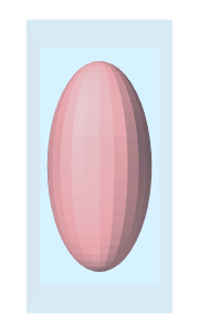
For simple shapes such as beams and ellipsoids, there are factory methods to automatically build the node and element structure. These methods are found in the FemFactory class. Some common methods are
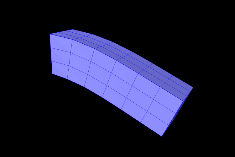
The inputs specify the dimensions, resolution, and potentially the type of element to use. The following code creates a basic beam made up of hexahedral elements:
1.2.2 Loading external FEM meshes
For more complex geometries, volumetric meshes can be loaded from external files. A list of supported file types is provided in Table 1.3. To load a geometry, an appropriate file reader must be created. Readers capable of reading FEM models implement the interface FemReader, which has the method
Additionally, many FemReader classes have static methods to handle the loading of files for convenience.
| Format | File extensions | Reader | Writer |
|---|---|---|---|
| ANSYS | .node, .elem | AnsysReader | AnsysWriter |
| TetGen | .node, .ele | TetGenReader | TetGenWriter |
| Abaqus | .inp | AbaqusReader | AbaqusWriter |
| VTK (ASCII) | .vtk | VtkAsciiReader | – |
The following code snippet demonstrates how to load a model using the AnsysReader.
The method PathFinder.getSourceRelativePath() is used to find a path within the ArtiSynth source tree that is relative to the current model’s source file (Section LABEL:PathFinder:sec). Note the try-catch block. Most of these readers throw an IOException if the read fails.
1.2.3 Generating from surfaces
There are two ways an FEM model can be generated from a surface: by using a FEM mesh generator, and by extruding a surface along its normal direction.
ArtiSynth has the ability to interface directly with the TetGen library (http://tetgen.org) to create a tetrahedral volumetric mesh given a closed and manifold surface. The main Java class for calling TetGen directly is TetgenTessellator. The tessellator has several advanced options, allowing for the computation of convex hulls, and for adding points to a volumetric mesh. For simply creating an FEM from a surface, there is a convenience routine within FemFactory that handles both mesh generation and constructing a FemModel3d:
If quality ![]() , then points will be added in an attempt to bound the
maximum radius-edge ratio (see the -q switch for TetGen). According
to the TetGen documentation, the algorithm usually succeeds for a
quality ratio of 1.2.
, then points will be added in an attempt to bound the
maximum radius-edge ratio (see the -q switch for TetGen). According
to the TetGen documentation, the algorithm usually succeeds for a
quality ratio of 1.2.
It’s also possible to create thin layer of elements by extruding a surface along its normal direction.
For example, to create a two-layer slice of elements centered about a surface of a tendon mesh, one might use
For this type of extrusion, triangular faces become wedge elements, and quadrilateral faces become hexahedral elements.
Note: for extrusions, no care is taken to ensure element quality; if the surface has a high curvature relative to the total extrusion thickness, then some elements will be inverted.
1.2.4 Building elements in code
A finite element model’s structure can also be manually constructed in code. FemModel3d has the methods:
For an element to successfully be added, all its nodes must already have been added to the model. Nodes can be constructed from a 3D location, and elements from an array of nodes. A convenience routine is available in FemElement3d that automatically creates the appropriate element type given the number of nodes (Table 1.1):
Be aware of node orderings when supplying nodes. For linear elements, ArtiSynth uses a clockwise convention with respect to the outward normal for the first face, followed by the opposite node(s). To determine the correct ordering for a particular element, check the coordinates returned by the function FemElement3dBase.getNodeCoords(). This returns the concatenated coordinate list for an “ideal” element of the given type.
1.2.5 Example: a simple beam model
A complete application model that implements a simple FEM beam is given below.
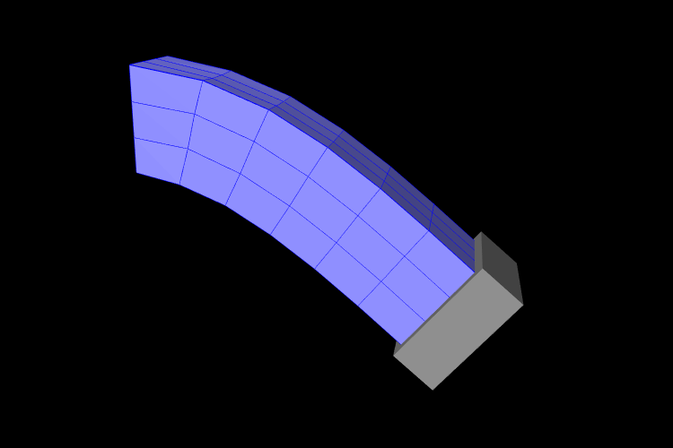
This example can be found in artisynth.demos.tutorial.FemBeam. The build() method first creates a MechModel and FemModel3d. A FEM beam is created using a factory method on line 36. This beam is centered at the origin, so its length extends from -length/2 to length/2. The density, damping and material properties are then assigned.
On lines 45–49, a fixed boundary condition is set to the left-hand side of the beam by setting the corresponding nodes to be non-dynamic. Due to numerical precision, a small EPSILON buffer is required to ensure all left-hand boundary nodes are identified (line 46).
Rendering properties are then assigned to the FEM model on line 52. These will be discussed further in Section 1.12.
1.3 FEM Geometry
Associated with each FEM model is a list of geometry with the heading meshes. This geometry can be used for either display purposes, or for interactions such as collisions (Section LABEL:CompoundCollidablesAndSelf:sec). A geometry itself has no physical properties; its motion is entirely governed by the FEM model that contains it.
All FEM geometries are of type FemMeshComp, which stores a reference to a mesh object (Section LABEL:Meshes:sec), as well as attachment information that links vertices of the mesh to points within the FEM. The attachments enforce the shape function interpolation in Equation (1.2) to hold at each mesh vertex, with constant shape function coefficients.
1.3.1 Surface meshes
By default, every FemModel3d has an auto-generated geometry representing the “surface mesh”. The surface mesh consists of all un-shared element faces (i.e. the faces of individual elements that are exposed to the world), and its vertices correspond to the nodes that make up those faces. As the FEM nodes move, so do the mesh vertices due to the attachment framework.
The surface mesh can be obtained using one of the following functions in FemModel3d:
The first returns the surface complete with attachment information. The latter method directly returns the PolygonalMesh that is controlled by the FEM.
It is possible to manually set the surface mesh:
However, doing so is normally not necessary. It is always possible to add additional mesh geometries to a finite element model, and the visibility settings can be changed so that the default surface mesh is not rendered.
1.3.2 Embedding geometry within an FEM
Any geometry of type MeshBase can be added to a FemModel3d. To do so, first position the mesh so that its vertices are in the desired locations inside the FEM, then call one of the FemModel3d methods:
The latter is a convenience routine that also gives the newly embedded FemMeshComp a name.
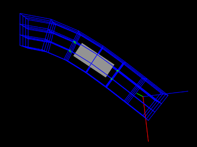
1.3.3 Example: a beam with an embedded sphere
A complete model demonstrating embedding a mesh is given below.
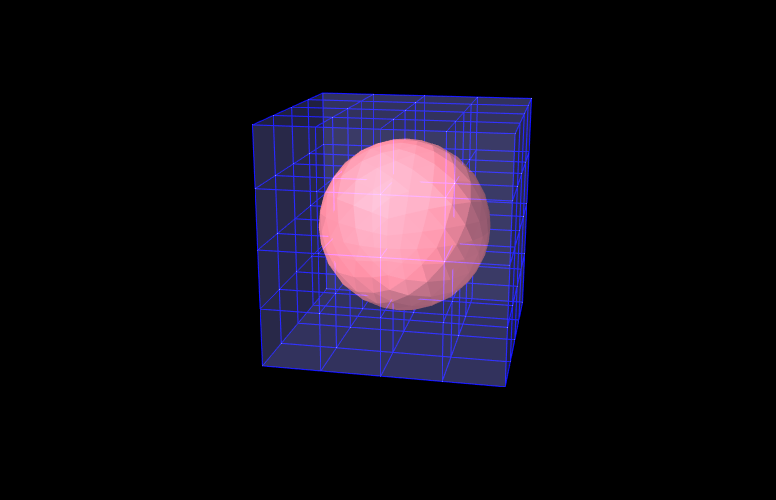
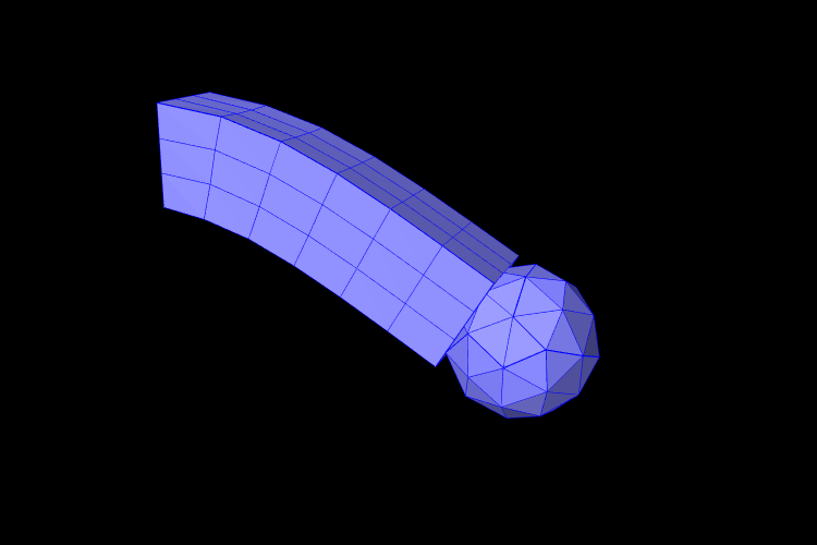
This example can be found in artisynth.demos.tutorial.FemEmbeddedSphere. The model is very similar to FemBeam. A MechModel and FemModel3d are created and added. At line 41, a PolygonalMesh of a sphere is created using a factory method. The sphere is already centered inside the beam, so it does not need to be repositioned. At Line 42, the sphere is embedded inside model fem, creating a FemMeshComp with the name “sphere”. The full model is shown in Figure 1.5.
1.4 Connecting FEM models to other components
To couple FEM models to other dynamic components, the “attachment” mechanism described in Section LABEL:PhysicsSimulation:sec is used. This involves creating and adding to the model attachment components, which are instances of DynamicAttachment, as described in Section LABEL:Attachments:sec. Common point-based attachment classes are listed in Table 1.4.
| Attachment | Description |
|---|---|
| PointParticleAttachment | Attaches one “point” to one “particle” |
| PointFrameAttachment | Attaches one “point” to one “frame” |
| PointFem3dAttachment | Attaches one “point” to a linear combination of FEM nodes |
FEM models are connected to other model components by attaching their nodes to various components. This can be done by creating an attachment object of the appropriate type, and then adding it to the MechModel using
There are also convenience routines inside MechModel that will create the appropriate attachments automatically (see Section LABEL:sec:mech:pointattachments).
All attachments described in this section are based around FEM nodes. However, it is also possible to attach frame-based components (such as rigid bodies) directly to an FEM, as described in Section 1.6.
1.4.1 Connecting nodes to rigid bodies or particles
Since FemNode3d is a subclass of Particle, the same methods described in Section LABEL:sec:mech:pointattachments for attaching particles to other particles and frames are available. For example, we can attach an FEM node to a rigid body using a either a statement of the form
or the following equivalent statement which does the same thing:
Both of these create a PointFrameAttachment between a rigid body (called body) and an FEM node (called node) and then adds it to the MechModel mech.
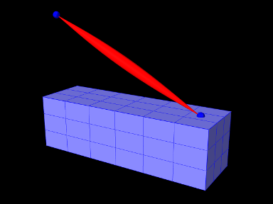
1.4.2 Example: connecting a beam to a block
The following model demonstrates attaching an FEM beam to a rigid block.
This model extends the FemBeam example of Section 1.2.5. The build() method then creates and adds a RigidBody block (lines 18–20). On line 21, the block is repositioned to the side of the beam to prepare for the attachment. On lines 24–28, all right-most nodes of the beam are then set to be attached to the block using a PointFrameAttachment. In this case, the attachments are explicitly created. They could also have been attached using
1.4.3 Connecting nodes directly to elements
Typically, nodes do not align in a way that makes it
possible to connect them to other FEM models and/or points based on
simple point-to-node attachments. Instead, we use a different
mechanism that allows us to attach a point to an arbitrary location
within an FEM model. This is done using an attachment component of
type
PointFem3dAttachment, which
implements an attachment where the position ![]() and velocity
and velocity ![]() of the
attached point is determined by a weighted sum of the positions
of the
attached point is determined by a weighted sum of the positions ![]() and velocities
and velocities ![]() of selected fem nodes:
of selected fem nodes:
| (1.3) |
Any force ![]() acting on the attached point is then propagated back
to the nodes, according to the relation
acting on the attached point is then propagated back
to the nodes, according to the relation
| (1.4) |
where ![]() is the force acting on node
is the force acting on node ![]() due to
due to ![]() . This
relation can be derived based on the conservation of energy.
If
. This
relation can be derived based on the conservation of energy.
If ![]() is embedded within a single element, then the
is embedded within a single element, then the ![]() are
simply the element nodes and the
are
simply the element nodes and the ![]() are corresponding shape
function values; this is known as an element-based attachment.
On the other hand, as described below, it is sometimes desirable to
form an attachment using a more general set of nodes that extends
beyond a single element; this is known as a nodal-based
attachment (Section 1.4.8).
are corresponding shape
function values; this is known as an element-based attachment.
On the other hand, as described below, it is sometimes desirable to
form an attachment using a more general set of nodes that extends
beyond a single element; this is known as a nodal-based
attachment (Section 1.4.8).
An element-based attachment can be created using a code fragment of the form
First, a PointFem3dAttachment is created for the point pnt. Next, setFromElement() is used to determine the nodal weights within the element elem for the specified position (which in this case is simply the point’s current position). To do this, it computes the “natural coordinates” coordinates of the position within the element. For this to be guaranteed to work, the position should be on or inside the element. If natural coordinates cannot be found, the method will return false and the nearest estimates coordinates will be used instead. However, it is sometimes possible to find natural coordinates outside a given element as long as the shape functions are well-defined. Finally, the attachment is added to the model.
More conveniently, the exact same functionality is provided by the attachPoint() method in MechModel:
This creates an attachment identical to that created by the previous code fragment.
Often, one does not want to have to determine the element to which a point should be attached. In that case, one can call
or, equivalently,
This will find the nearest element to the node in question and use that to create the attachment. If the node is outside the FEM model, then it will be attached to the nearest point on the FEM’s surface.
1.4.4 Example: connecting two FEMs together
The following model demonstrates how to attach two FEM models together:
This example can be found in artisynth.demos.tutorial.FemBeamWithFemSphere. The model extends FemBeam, adding a finite element sphere and coupling them together. The sphere is created and added on lines 18–28. It is read from TetGen-generated files using the TetGenReader class. The model is then scaled to match the dimensions of the current model, and transformed to the right side of the beam. To create attachments, the code first checks for any nodes that belong to the sphere that fall inside the beam using the FemModel3d.findContainingElement(Point3d) method (line 36), which returns the containing element if the point is inside the model, or null if the point is outside. Internally, this spatial search uses a bounding volume hierarchy for efficiency (see BVTree and BVFeatureQuery). If the point is contained within the beam, then mech.attachPoint() is used to attach it to the nodes of the element (line 39).
1.4.5 Finding which nodes to attach
While it is straightforward to connect nodes to rigid bodies or other FEM nodes or elements, it is often necessary to determine which nodes to attach. This was evident in the example of Section 1.4.4, which attached nodes of an FEM sphere that were found to be inside an FEM beam.
As in that example, finding the nodes to attach can often be done using geometric queries. For example, we often select nodes based on how close they are to the other body we wish to attach to.
Various prolixity queries are available for this task. To find the distance of a point to a polygonal mesh, we can use the following PolygonalMesh methods,
| double distanceToPoint(Point3d pnt) |
Returns the distance of pnt to the mesh. |
| int pointIsInside (Point3d pnt) |
Returns true if pnt is inside the mesh. |
where the latter method returns 1 if the point is inside and 0 otherwise. For checking the distance of an FEM node, pnt can be obtained from node.getPosition() (or possibly node.getRestPosition()). For example, to find all nodes within a distance tol of the surface of a rigid body, we could use the code fragment:
If we want to check only nodes that lie on the FEM surface, then we can filter them using the FemModel3d method isSurfaceNode():
Most of the mesh-based query methods work only for triangular meshes. The PolygonalMesh method isTriangular() can be used to determine if the mesh is triangular. If it is not, it can made triangular by calling triangulate(), although in general this should be done during model construction before the mesh-based component has been added to the model.
For connecting an FEM model to another FEM model, FemModel3d provides a number of query methods:
| Nearest element queries: | |
|---|---|
| FemElement3dBase findNearestElement( Point3d near, Point3d pnt) |
Find nearest element (shell or volumetric) to pnt. |
| FemElement3dBase findNearestElement( Point3d near, Point3d pnt, ElementFilter filter) |
Find nearest filtered element (shell or volumetric) to pnt. |
| FemElement3dBase findNearestSurfaceElement( Point3d near, Point3d pnt) |
Find nearest surface element (shell or volumetric) to pnt. |
| FemElement3d findNearestVolumetricElement ( Point3d near, Point3d pnt) |
Find nearest volumetric element to pnt. |
| ShellElement3d findNearestShellElement ( Point3d near, Point3d pnt) |
Find nearest shell element to pnt. |
| FemElement3d findContainingElement(Point3d pnt) |
Find volumetric element (if any) containing pnt. |
| Nearest node queries: | |
|---|---|
| FemNode3d findNearestNode ( Point3d pnt, double maxDist) |
Find nearest node to pnt that is within maxDist. |
| ArrayList<FemNode3d> findNearestNodes ( Point3d pnt, double maxDist) |
Find all nodes that are within maxDist of pnt. |
All the above queries are based on the FEM model’s current nodal
positions. The method
findNearestElement(near,pnt,filter) allows the application to
specify
a FemModel.ElementFilter to
restrict the elements that are searched.
The argument near that appears in some of the queries is an optional argument which, if not null, returns the location of the corresponding nearest point on the element. The distance from pnt to the element can then be found using
near.distance (pnt);
If the resulting distance is 0, then the point is on or inside the element. Otherwise, the point is outside the element, and if no element filters were used in the query, outside the FEM model itself.
Typically, it is preferred attach a point to an element only if it lies on or inside an element. However, it is possible to attach points outside an element as long as the system is able to determine appropriate element “coordinates” for that point (which it may not be able to do if the point is far away). In addition, the motion behavior of an exterior attached point may sometimes appear counterintuitive.
The FemModel3d element and node queries can be used in a variety of ways.
findNearestNodes() can be used to find all nodes within a certain distance of a point, as part of the process of making nodal-based attachments (Section 1.4.8).
findNearestNode() is used in the FemMuscleBeam example (Section 1.9.5) to determine if a desired muscle point is near enough to a node to use that node directly, or if a marker should be created.
As another example, suppose we wish to connect the surface nodes of an FEM model femA to the surface elements of another model femB if they lie within a prescribed distance tol of the surface of femB. Then we could use the following code:
Finally, it is possible to identify nodes on the surface of an FEM model according to whether they belong to specific features, such as a smooth patch or a sharp edge line. Methods for doing this are provided as static methods in the class FemQuery, and include:
| Feature based node queries: | |
|---|---|
| ArrayList<FemNode3d> findPatchNodes ( FemModel3d fem, FemNode3d node0, double maxBendAng) |
Find nodes in patch defined by a maximum bend angle. |
| ArrayList<FemNode3d> findPatchBoundaryNodes ( FemModel3d fem, FemNode3d node0, double maxBendAng) |
Find the border nodes of a patch. |
| ArrayList<FemNode3d> findEdgeLineNodes ( FemModel3d fem, FemNode3d node0, double minBendAng, double maxEdgeAng, double allowBranching) |
Find the nodes along an edge defined by a minimum bend angle. |
Details of how these methods work are given in their API documentation. They use the notion of a bend angle, which is the absolute value of the angle between two faces about their common edge. A patch is defined by a collection of faces whose bend angles do not exceed a minimum value, while an edge line is a collection of edges with bend angles not below a maximum value. The feature methods start with an initial node (node0) and then grow the requested feature out from there. For example, suppose we have a regular hexahedral FEM grid, and we wish to find all the nodes on one of the faces. If we know one of the nodes on the face, then we can find all of the nodes using findPatchNodes:
Note that the feature query above uses a maximum bend angle of
![]() . Because grid faces are flat, this choice is somewhat
arbitrary; any angle larger than 0 (within machine precision) would also
work.
. Because grid faces are flat, this choice is somewhat
arbitrary; any angle larger than 0 (within machine precision) would also
work.
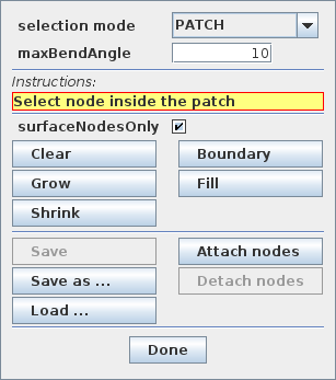
1.4.6 Selecting nodes in the viewer
Often, it is most convenient to select nodes in the ArtiSynth viewer. For this, a node selection tool is available (Figure 1.8), as described in the section “Selecting FEM nodes” of the ArtiSynth User Interface Guide). It allows nodes to be selected in various ways, including the usual click, drag box and elliptical selection tools, as well as specialized operations that select nodes based on patches, edge lines, and distances to other bodies. Once nodes have been selected, their numbers can be saved to a node number file which can then be read by a model’s build() method to determine which nodes to connect to some body.
Node number files are text files with a very simple format, consisting of integers (the node numbers), separated by white space. There is no limit to how many numbers can appear on a line but typically this is limited to ten or so to make the file more readable. Optionally, the numbers can be surrounded by square brackets ([ ]). The special character ‘#’ is a comment character, commenting out all characters from itself to the end of the current line. For a file containing the node numbers 2, 12, 4, 8, 23 and 47, the following formats are all valid:
Once node numbers have been identified in the viewer and saved in a file, they can be read by the build() method using a NodeNumberReader. For convenience, this class supplies two static methods for extracting the FEM nodes specified by the numbers in a file:
| static ArrayList<FemNode3d> read( File file, FemModel3d fem) |
Returns nodes in fem corresponding to file’s numbers. |
| static ArrayList<FemNode3d> read( String filePath, FemModel3d fem) |
Returns nodes in fem corresponding to file’s numbers. |
Extracted nodes can be used to set boundary conditions or form connections with other bodies. For example, suppose we wish to connect a face of an FEM model fem to a rigid body block, using a set of nodes specified in a file called faceNodes.txt. A code fragment to accomplish this could be the following:
The process of selecting nodes in the viewer, saving them in a file, and using them in a model can be done iteratively: if the selected nodes need to be adjusted, one can reopen the node selection tool, load the selection from file, adjust the selection, and resave the file, without needing to make any modifications to the model’s build() code.
If desired, one can also determine a set of nodes in code, and then write their numbers to a file using the class NodeNumberWriter, which supplies static methods for writing number files:
| static void write( String filePath, Collection<FemNode3d> nodes) |
Writes the numbers of nodes to the specified file. |
| static void write( File file, Collection<FemNode3d> nodes) |
Writes the numbers of nodes to file. |
| static void write( File file, Collection<FemNode3d> nodes, int maxCols, int flags) |
Writes the numbers of nodes to file, using the specified number of columns and format flags. |
For example:
1.4.7 Example: two bodies connected by an FEM “spring”
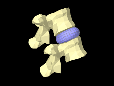
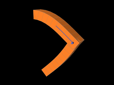
The LumbarFrameSpring example in Section LABEL:LumbarFrameSpring:sec uses a frame spring to connect two simplified lumbar vertebrae. However, it is also possible to use an FEM model in place of a frame spring, possibly providing a more realistic model of the intervertebral disc. A simple model which does this is defined in
artisynth.demos.tutorial.LumbarFEMDisk
The initial source code is similar to that for LumbarFrameSpring, but differs in the section where the FEM disk replaces the FrameSpring:
The simplified FEM model representing the “disk” is created at lines 57-61, using a torus-shaped model created by FemFactory. It is then repositioning using transformGeometry() ( Section LABEL:TransformingGeometry:sec) to place it between the vertebrae (line 64-66). After the FEM model is positioned, we find which nodes are within a distance tol of each vertebral surface and attach them to the appropriate body (lines 69-81).
To run this example in ArtiSynth, select All demos > tutorial > LumbarFEMDisk from the Models menu. The model should load and initially appear as in Figure 1.9. The behavior is best seem by running the model and using the pull controller to exert forces on the upper vertebra.
1.4.8 Nodal-based attachments
The example of Section 1.4.4 uses element-based attachments to connect the nodes of one FEM to elements of another. As mentioned above, element-based attachments assume that the attached point is associated with a specific FEM model element. While this often gives good results, there are situations where it may be desirable to distribute the connection more broadly among a larger set of nodes.
In particular, this is sometimes the case when connecting FEM models to point-to-point springs. The end-point of such a spring may end up exerting a large force on the FEM, and then if the number of nodes to which the end-point is attached are too small, the resulting forces on these nodes (Equation 1.4) may end up being too large. In other words, it may be desirable to distribute the spring’s force more evenly throughout the FEM model.
To handle such situations, it is possible to create a nodal-based attachment in which the nodes and weights are explicitly specified. This involves explicitly creating a PointFem3dAttachment for the point or particle to be attached and the specifying the nodes and weights directly,
where nodes and weights are arrays of FemNode and double, respectively. It is up to the application to determine these.
PointFem3dAttachment provides several methods for explicitly specifying nodes and weights. The signatures for these include:
The last two methods determine the weights automatically, using an
inverse-distance-based calculation in which each weight ![]() is initially computed as
is initially computed as
| (1.4) |
where ![]() is the distance from node
is the distance from node ![]() to pos and
to pos and
![]() is the maximum distance. The weights are then
adjusted to ensure that they sum to one and that the weighted sum of
the nodes equals pos. In some cases, the specified nodes
may not provide enough support for the last condition to be
met, in which case the methods return false.
is the maximum distance. The weights are then
adjusted to ensure that they sum to one and that the weighted sum of
the nodes equals pos. In some cases, the specified nodes
may not provide enough support for the last condition to be
met, in which case the methods return false.
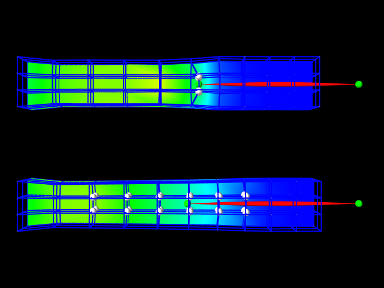
1.4.9 Example: element vs. nodal-based attachments
The model demonstrating the difference between element and nodal-based attachments is defined in
artisynth.demos.tutorial.PointFemAttachment
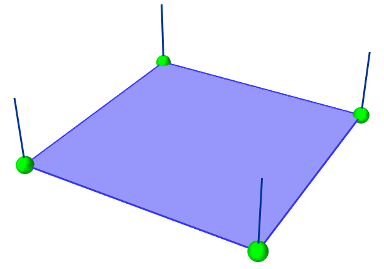
It creates two FEM models, each with a single point-to-point spring attached to a particle at their center. The model at the top (fem1 in the code below) is connected to the particle using an element-based attachment, while the lower model (fem2 in the code) is connected using a nodal-based attachment with a larger number of nodes. Figure 1.10 shows the result after the model is run until stable. The element-based attachment results in significantly higher deformation in the immediate vicinity around the attachment, while for the nodal-based attachment, the deformation is distributed much more evenly through the model.
The build method and some of the auxiliary code for this model is shown below. Code for the other auxiliary methods, including addFem(), addParticle(), addSpring(), and setAttachedNodesWhite(), can be found in the actual source file.
The build() method begins by creating a MechModel and then adding to it two FEM beams (created using the auxiliary method addFem(). Rendering of each FEM model’s surface is then set up to show strain values (setSurfaceRendering(), lines 41 and 43). The surface meshes themselves are also redefined to exclude the frontmost elements, allowing the strain values to be displayed closer model centers. This redefinition is done using calls to createSurfaceMesh() (lines 40, 41) with a custom ElementFilter defined at lines 3-12.
Next, the end-point particles for the axial springs are created (using the auxiliary method addParticle(), lines 46-49), and particle m1 is attached to fem1 using mech.attachPoint() (line 52), which creates an element-based attachment at the point’s current location. Point m2 is then attached to fem2 using a nodal-based attachment. The nodes for these are collected as the union of all nodes for a specified set of elements (lines 58-59, and the method collectNodes() defined at lines 16-25). These are then used to create a nodal-based attachment (lines 61-63), where the weights are determined automatically using the method associated with equation (1.4).
Finally, the springs are created (auxiliary method addSpring(), lines 66-67), the nodes associated for each attachment are set to render as white spheres (setAttachedNodesWhites(), lines 70-71), and the particles are set to render as green spheres.
To run this example in ArtiSynth, select All demos > tutorial > PointFemAttachment from the Models menu. Running the model will cause it to settle into the state shown in Figure 1.10. Selecting and dragging one of the spring anchor points at the right will cause the spring tension to vary and further illustrate the difference between the element and nodal-based attachments.
1.5 FEM markers
Just as there are FrameMarkers to act as anchor points on a frame or rigid body (Section LABEL:FrameMarkers:sec), there are also FemMarkers that can mark a point inside a finite element. They are frequently used to provide anchor points for attaching springs and forces to a point inside an element, but can also be used for graphical purposes.
FEM markers are implemented by the class FemMarker, which is a subclass of Point. They are essentially massless points that contain their own attachment component, so when creating and adding a marker there is no need to create a separate attachment component.
Within the component hierarchy, FEM markers are typically stored in the markers list of their associated FEM model. They can be created and added using a code fragment of the form
This creates a marker at the location ![]() (in world
coordinates), calls setFromFem() to attach it to the nearest
element in the FEM model ( which is either the containing element or
the nearest element on the model’s surface), and then adds it to the
markers list.
(in world
coordinates), calls setFromFem() to attach it to the nearest
element in the FEM model ( which is either the containing element or
the nearest element on the model’s surface), and then adds it to the
markers list.
If the marker’s attachment has not already been set when addMarker() is called, then addMarker() will call setFromFem() automatically. Therefore the above code fragment is equivalent to the following:
Alternatively, one may want to explicitly specify the nodes associated with the attachment, as described in Section 1.4.8:
There are a variety of methods available to set the attachment, mirroring those available in the underlying base class PointFem3dAttachment:
The last two methods compute nodal weights automatically, as described in Section 1.4.8, based on the marker’s currently assigned position. If the supplied nodes do not provide sufficient support, then the methods return false.
Another set of convenience methods are supplied by FemModel3d, which combine these with the addMarker() call:
For example, one can do
Markers are often used to track movement within an FEM model. For that, one can examine their positions and velocities, as with any other particles, using the methods
The return values from these methods should not be
modified. Alternatively, when a 3D force ![]() is applied to the
marker, it is distributed to the attached nodes according to the nodal
weights, as described in Equation (1.4).
is applied to the
marker, it is distributed to the attached nodes according to the nodal
weights, as described in Equation (1.4).
1.5.1 Example: attaching an FEM beam to a muscle
A complete application model that employs a fem marker as an anchor for a spring is given below.
This example can be found in artisynth.demos.tutorial.FemBeamWithMuscle. This model extends the FemBeam example, adding a FemMarker for the spring to attach to. The method createMarker(...) on lines 29–35 is used to create and add a marker to the FEM. Since the element is initially set to null, when it is added to the FEM, the model searches for the containing or nearest element. The loaded model is shown in Figure 1.11.
1.6 Frame attachments
It is also possible to attach frame components, including rigid bodies, directly to FEM models, using the attachment component FrameFem3dAttachment. Analogously to PointFem3dAttachment, the attachment is implemented by connecting the frame to a set of FEM nodes, and attachments can be either element-based or nodal-based. The frame’s origin is computed in the same way as for point attachments, using a weighted sum of node positions (Equation 1.3), while the orientation is computed using a polar decomposition on a deformation gradient determined from either element shape functions (for element-based attachments) or a Procrustes type analysis using nodal rest positions (for nodal-based attachments).
An element-based attachment can be created using either a code fragment of the form
or, equivalently, the attachFrame() method in MechModel:
This attaches the frame frame to the nodes of the FEM element elem. As with PointFem3dAttachment, if the frame’s origin is not inside the element, it may not be possible to accurately compute the internal nodal weights, in which case setFromElement() will return false.
In order to have the appropriate element located automatically, one can instead use
or, equivalently,
As with point-to-FEM attachments, it may be desirable to create a nodal-based attachment in which the nodes and weights are not tied to a specific element. The reasons for this are generally the same as with nodal-based point attachments (Section 1.4.8): the need to distribute the forces and moments acting on the frame across a broader set of element nodes. Also, element-based frame attachments use element shape functions to determine the frame’s orientation, which may produce slightly asymmetric results if the frame’s origin is located particularly close to a specific node.
FrameFem3dAttachment provides several methods for explicitly specifying nodes and weights. The signatures for these include:
Unlike their counterparts in PointFem3dAttachment, the first two methods also require the current desired pose of the frame TFW (in world coordinates). This is because while nodes and weights will unambiguously specify the frame’s origin, they do not specify the desired orientation.
1.6.1 Example: attaching frames to an FEM beam
A model illustrating how to connect frames to an FEM model is defined in
artisynth.demos.tutorial.FrameFemAttachment
It creates an FEM beam, along with a rigid body block and a massless coordinate frame, that are then attached to the beam using nodal and element-based attachments. The build method is shown below:
Lines 3-22 create a MechModel and populate it with an FEM beam and a rigid body box. Next, a basic Frame is created, with a specified pose and an axis length of 0.3 (to allow it to be seen), and added to the MechModel (lines 25-28). It is then attached to the FEM beam using an element-based attachment (line 30). Meanwhile, the box is attached to using a nodal-based attachment, created from all the nodes associated with elements 22 and 31 (lines 33-36). Finally, all attachment nodes are set to be rendered as green spheres (lines 39-41).
To run this example in ArtiSynth, select All demos > tutorial > FrameFemAttachment from the Models menu. Running the model will cause it to settle into the state shown in Figure 1.12. Forces can interactively be applied to the attached block and frame using the pull tool, causing the FEM model to deform (see the section “Pull Manipulation” in the ArtiSynth User Interface Guide).
1.6.2 Adding joints to FEM models
The ability to connect frames to FEM models, as described in Section 1.6, makes it possible to interconnect different FEM models directly using joints, as described in Section LABEL:JointsAndConnectors:sec. This is done internally by using FrameFem3dAttachments to connect frames C and D of the joint (Figure LABEL:jointExample:fig) to their respective FEM models.
As indicated in Section LABEL:CreatingJoints:sec, most joints have a constructor of the form
that creates a joint connecting bodyA to bodyB, with the initial pose of the D frame given (in world coordinates) by TDW. The same body and transform settings can be made on an existing joint using the method setBodies(bodyA, bodyB, TDW). For these constructors and methods, it is possible to specify FEM models for bodyA and/or bodyB. Internally, the joint then creates a FrameFem3dAttachment to connect frame C and/or D of the joint (See Figure LABEL:jointExample:fig) to the corresponding FEM model.
However, unlike joints involving rigid bodies or frames, there are no
associated ![]() or
or ![]() transforms (since there is no fixed
frame within an FEM to define such transforms). Methods or
constructors which utilize
transforms (since there is no fixed
frame within an FEM to define such transforms). Methods or
constructors which utilize ![]() or
or ![]() can therefore
not be used with FEM models.
can therefore
not be used with FEM models.
1.6.3 Example: two FEM beams connected by a joint
A model connecting two FEM beams by a joint is defined in
artisynth.demos.tutorial.JointedFemBeams
It creates two FEM beams and connects them via a special slotted-revolute joint. The build method is shown below:
Lines 3-16 create a MechModel and populates it with two FEM beams, fem1 and fem2, using an auxiliary method addFem() defined in the model source file. The leftmost nodes of fem1 are set fixed. A SlottedRevoluteJoint is then created to interconnect fem1 and fem2 at a location specified by TDW (lines 19-21). Lines 24-29 set some parameters for the joint, along with various render properties.
To run this example in ArtiSynth, select All demos > tutorial > JointedFemBeams from the Models menu. Running the model will cause it drop and flex under gravity, as shown in 1.13. Forces can interactively be applied to the beams using the pull tool (see the section “Pull Manipulation” in the ArtiSynth User Interface Guide).
1.7 Incompressibility
FEM incompressibility within ArtiSynth is enforced by trying to ensure that the volume of an FEM remains locally constant. This, in turn, is accomplished by constraining nodal velocities so that the local volume change, or divergence, is zero (or close to zero). There are generally two ways to do this:
-
•
Hard incompressibility, which sets up explicit constraints on the nodal velocities;
-
•
Soft incompressibility, which uses a restoring pressure based on a potential field to try to keep the volume constant.
Both of these methods operate independently, and both can be used either separately or together. Generally speaking, hard incompressibility will result in incompressibility being more rigorously enforced, but at the cost of increased computation time and (sometimes) less stability. Soft incompressibility allows the application to control the restoring force used to enforce incompressibility, usually by adjusting the value of the bulk modulus material property. As the bulk modulus is increased, soft incompressibility starts to act more like ‘hard’ incompressibility, with an infinite bulk modulus corresponding to perfect incompressibility. However, very large bulk modulus values will generally produce stability problems.
Incompressibility is not currently implemented for shell elements. Applying hard incompressibility to a shell element will have no effect on its behavior. If soft incompressibility is applied, by supplying the element with an incompressible material, then only the deviatoric component of that material will have any effect; the dilational component will generate no stress.
1.7.1 Volume regions and locking
Both hard and soft incompressibility can be applied to different regions of local volume. From larger to smaller, these regions are:
-
•
Nodal - the local volume surrounding each node;
-
•
Element - the volume of each element;
-
•
Full - the volume at each integration point.
Element-based incompressibility is the standard method generally seen
in the literature. However, it tends not to work well for
tetrahedral meshes, because constraining the volume of each tet in a
tetrahedral mesh tends to over constrain the system. This is because
the number of tets in a large tetrahedral mesh is often ![]() ,
where
,
where ![]() is the number of nodes, and so putting a volume constraint
on each element may result in
is the number of nodes, and so putting a volume constraint
on each element may result in ![]() constraints, which exceeds the
constraints, which exceeds the
![]() degrees of freedom (DOF) in the FEM. This overconstraining results in an
artificially increased stiffness known as locking. Because of
locking, for tetrahedrally based meshes it may be better to use
nodal-based incompressibility, which creates a single volume constraint
around each node, resulting in only
degrees of freedom (DOF) in the FEM. This overconstraining results in an
artificially increased stiffness known as locking. Because of
locking, for tetrahedrally based meshes it may be better to use
nodal-based incompressibility, which creates a single volume constraint
around each node, resulting in only ![]() constraints, leaving
constraints, leaving ![]() DOF
to handle the remaining deformation. However, nodal-based
incompressibility is computationally more costly than element-based
and may not be as stable.
DOF
to handle the remaining deformation. However, nodal-based
incompressibility is computationally more costly than element-based
and may not be as stable.
Generally, the best solution for incompressible problems is to use
element-based incompressibility with a mesh consisting of hexahedra,
or primarily hexahedra and a mix of other elements (the latter
commonly being known as a hex dominant mesh). For hex-based
meshes, the number of elements is roughly equal to the number of
nodes, and so adding a volume constraint for each element imposes ![]() constraints on the model, which (like nodal incompressibility)
leaves
constraints on the model, which (like nodal incompressibility)
leaves ![]() DOF to handle the remaining deformation.
DOF to handle the remaining deformation.
Full incompressibility tries to control the volume at each integration point within each element, which almost always results in a large number of volumetric constraints and hence locking. It is therefore not commonly used and is provided mostly for debugging and diagnostic purposes.
1.7.2 Hard incompressibility
Hard incompressibility is controlled by the incompressible property of the FEM, which can be set to one of the following values of the enumerated type FemModel.IncompMethod:
- OFF
-
No hard incompressibility enforced.
- ELEMENT
-
Element-based hard incompressibility enforced (Section 1.7.1).
- NODAL
-
Nodal-based hard incompressibility enforced (Section 1.7.1).
- AUTO
-
Selects either ELEMENT or NODAL, with the former selected if the number of elements is less than or equal to the number of nodes.
- ON
-
Same as AUTO.
Hard incompressibility uses explicit constraints on the nodal velocities to enforce the incompressibility, which increases computational cost. Also, if the number of constraints is too large, perturbed pivot errors may be encountered by the solver. However, hard incompressibility can in principle handle situations where complete incompressibility is required. It is equivalent to the mixed u-P formulation used in commercial FEM codes (such as ANSYS), and the Lagrange multipliers computed for the constraints are pressure impulses.
Hard incompressibility can be applied in addition to soft incompressibility, in which case it will provide additional incompressibility enforcement on top of that provided by the latter. It can also be applied to linear materials, which are not themselves able to emulate true incompressible behavior (Section 1.7.4).
1.7.3 Soft incompressibility
Soft incompressibility enforces incompressibility using a restoring
pressure that is controlled by a volume-based energy potential. It is
only available for FEM materials that are subclasses of
IncompressibleMaterial.
The energy potential ![]() is a function of the determinant
is a function of the determinant ![]() of the
deformation gradient, and is scaled by the material’s bulk modulus
of the
deformation gradient, and is scaled by the material’s bulk modulus
![]() . The restoring pressure
. The restoring pressure ![]() is given by
is given by
| (1.5) |
Different potentials can be selected by setting the bulkPotential property of the incompressible material, whose value is an instance of IncompressibleMaterial.BulkPotential. Currently there are two different potentials:
- QUADRATIC
-
The potential and associated pressure are given by
(1.6) - LOGARITHMIC
-
The potential and associated pressure are given by
(1.7)
The default potential is QUADRATIC, which may provide slightly improved stability characteristics. However, we have not noticed significant differences between the two potentials in practice.
How soft incompressibility is applied within an FEM model is controlled by the FEM’s softIncompMethod property, which can be set to one of the following values of the enumerated type FemModel.IncompMethod:
- ELEMENT
-
Element-based soft incompressibility enforced (Section 1.7.1).
- NODAL
-
Nodal-based soft incompressibility enforced (Section 1.7.1).
- AUTO
-
Selects either ELEMENT or NODAL, with the former selected if the number of elements is less than or equal to the number of nodes.
- FULL
-
Incompressibility enforced at each integration point (Section 1.7.1).
1.7.4 Incompressibility and linear materials
Within a linear material, incompressibility is controlled by Poisson’s
ratio ![]() , which for isotropic materials can assume a value in the
range
, which for isotropic materials can assume a value in the
range ![]() . This specifies the amount of transverse contraction
(or expansion) exhibited by the material as it compressed or extended
along a particular direction. A value of
. This specifies the amount of transverse contraction
(or expansion) exhibited by the material as it compressed or extended
along a particular direction. A value of ![]() allows the material to be
compressed or extended without any transverse contraction or
expansion, while a value of
allows the material to be
compressed or extended without any transverse contraction or
expansion, while a value of ![]() in theory indicates a perfectly
incompressible material. However, setting
in theory indicates a perfectly
incompressible material. However, setting ![]() in practice
causes a division by zero, so only values close to 0.5 (such as 0.49)
can be used.
in practice
causes a division by zero, so only values close to 0.5 (such as 0.49)
can be used.
Moreover, the incompressibility only applies to small displacements,
so that even with ![]() it is still possible to squash a linear
FEM completely flat if enough force is applied. If true incompressible
behavior is desired with a linear material, then one must also use
hard incompressibility (Section 1.7.2).
it is still possible to squash a linear
FEM completely flat if enough force is applied. If true incompressible
behavior is desired with a linear material, then one must also use
hard incompressibility (Section 1.7.2).
1.7.5 Using incompressibility in practice
As mentioned above, when modeling incompressible models, we have found that the best practice is to use, if possible, either a hex or hex-dominant mesh, along with element-based incompressibility.
Hard incompressibility allows the handling of full incompressibility but at the expense of greater computational cost and often less stability. When modeling biomechanical materials, it is often permissible to use only soft incompressibility, partly since biomechanical materials are rarely completely incompressible. When implementing soft incompressibility, it is common practice to set the bulk modulus to something like 100 times the other (deviatoric) stiffnesses of the material.
We have found stability behavior to be complex, and while hard incompressibility often results in less stable behavior, this is not always the case: in some situations the stronger enforcement afforded by hard incompressibility actually improves stability.
1.8 Varying and augmenting material behaviors
The default material used by all elements of an FEM model is supplied by the model’s material property. However, it is often the case that one wishes to specify different material behaviors for different sets of elements within an FEM model. This may be particularly true when combining volumetric and shell elements.
There are several ways to vary material behavior within a model. These include:
-
•
Setting an explicit material for specific elements, using their material property. An element’s material is null by default, but if set to a material, it will override the default material supplied by the FEM model. While this method is quite straightforward, it does have one disadvantage: because material settings are copied by each element, subsequent interactive or online changes to the material require resetting the material in all the affected elements.
-
•
Binding one or more material parameters to a field. Sometimes certain material parameters, such as stiffness quantities or direction information, may need to vary across the FEM domain. While sometimes this can be handled by setting material properties for specific elements, it may be more convenient to bind the varying properties to a field, which can specify varying values over a domain composed of either a regular grid or an FEM mesh. Only one material needs to be used, and any properties which are not bound can be adjusted interactively or online. Fields and their bindings are described in detail in Chapter LABEL:sec:fields.
-
•
Adding augmenting material behaviors using MaterialBundles. A material bundle may be specified either for all elements, or for a subset of them, and each provides one material (via its own material property) whose behavior is added to that of the indicated elements. This also provides an easy way to combine the behaviors of two of more materials in the same element. One also has the option of setting the material property of the certain elements to NullMaterial, so that only the augmenting material(s) are applied.
-
•
Adding muscle behaviors using MuscleBundles. This is analogous to using MaterialBundles, except that MuscleBundles are restricted to using an instance of a MuscleMaterial, and include support for handling the excitation value, as well as the activation directions (which usually vary across the FEM domain). MuscleBundles are only present in the FemMuscleModels subclass of FemModel3d, and are described in detail in Section 1.9.
The remainder of this section will discuss MaterialBundles.
Adding a MaterialBundle to an FEM model is illustrated by the following code fragment:
Once added, the stress computed by the bundle’s material will be added to the stress computed by any other materials which are active for the bundle’s elements.
When deciding what elements to add to a bundle, one is free to choose any means necessary. The example above inspects all the volumetric elements in the FEM. To instead inspect all the shell elements, or all volumetric and shell elements, one could use the code fragments such as the following:
Of course, if the elements are known through other means, then they can be added directly.
The element composition of a bundle can be controlled by the methods
It is also possible to create a MaterialBundle whose material is added to all the FEM elements. This can done either by using one of the following constructors
with useAllElements set to true, or by calling the method
When a bundle is set to use all the FEM elements, it clears its own element list, and one is not permitted to add elements using addElement(elem).
After a bundle has been created, it is possible to get or set its material property using the methods
Again, because materials are copied internally, any modification to a material after it has been used as an input to setMaterial() will not be noticed by the bundle. Instead, one should modify the material before calling setMaterial(), or modify the copied material which can be obtained by calling getMaterial() or by storing the value returned by setMaterial().
Finally, a MuscleBundle is a renderable component. Setting its elementWidgetSize property to a value greater than zero will cause the rendering of all its elements, using a solid widget representation of each at a scale controlled by elementWidgetSize: 0.5 for half size, 1.0 for full size, etc. The color of the widgets is controlled by the faceColor property of the bundle’s renderProps. Being able to render the elements makes it easy to select the bundle and visualize which elements it contains.
1.8.1 Example: FEM sheet with a stiff spine
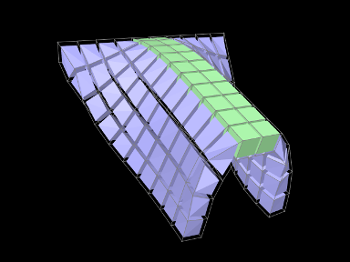
A simple model demonstrating the use of material bundles is defined in
artisynth.demos.tutorial.MaterialBundleDemo
It consists of a simple thin hexahedral sheet in which a material bundle is used to stiffen elements close to the x-axis, creating a stiff “spine”. While the same effect could be achieved by simply setting a different material property for the “spine” elements, it does provide a good example of muscle bundle usage. The model’s build method is given below:
Lines 6-9 create a thin FEM hex sheet, centered on the origin, with
size ![]() and
and ![]() elements
along each axis. Its material is set to a linear material with a
Young’s modulus of
elements
along each axis. Its material is set to a linear material with a
Young’s modulus of ![]() . The leftmost nodes are then fixed (lines
11-16).
. The leftmost nodes are then fixed (lines
11-16).
Next, a MuscleBundle is added and used to apply an additional
material to the elements near the x axis (lines 19-29). It is given a
neo-hookean material with a much higher stiffness, and the “spine”
elements for it are selected by finding those whose centroids
have a ![]() value within 0.1 of the x axis.
value within 0.1 of the x axis.
After the bundle is added, a control panel is created allowing interactive control of the materials for both the FEM model and the bundle, along with their elementWidgetSize properties.
Finally, some render properties are set (lines 41-44). The idea is to render the elements of both the FEM model and the bundle using element widgets (both of which will be visible since there is no surface rendering and the element widget sizes for both are greater than 0). The widget size for the bundle is made larger than that of the FEM model to ensure its widgets will cover those of the latter. Widget colors are controlled by the FEM and bundle face colors, set in lines 41-42.
The example can be run in ArtiSynth by selecting All demos > tutorial > MaterialBundleDemo from the Models menu. When it is run, the sheet will fall under gravity but be much stiffer along the spine (Figure 1.14). The control panel can be used to interactively adjust the material parameters for both the FEM and the bundle. This is one advantage of using bundles: the same material can be used to control multiple elements. The panel also allows interactive adjustment of the widget sizes, to illustrate what they look like and how they are rendered.
1.9 Muscle activated FEM models
Finite element muscle models are an extension to regular FEM models. As such, everything previously discussed for regular FEM models also applies to FEM muscles. Muscles have additional properties that allow them to contract when activated. There are two types of muscles supported:
- Fibre-based:
-
Point-to-point muscle fibres are embedded in the model.
- Material-based:
-
An auxiliary material is added to the constitutive law to embed muscle properties.
In this section, both types will be described.
1.9.1 FemMuscleModel
The main class for FEM-based muscles is FemMuscleModel, a subclass of FemModel3d. It differs from a basic FEM model in that it has the new property
| Property | Description |
| muscleMaterial | An object that adds an activation-dependent ‘muscle’ term to the constitutive law. |
This is a delegate object of type MuscleMaterial, described in detail in Section 1.10.3, that computes activation-dependent stress and stiffness in the muscle. In addition to this property, FemMuscleModel adds two new lists of subcomponents:
- bundles
-
Groupings of muscle sub-units (fibres or elements) that can be activated. - exciters
-
Components that control the activation of a set of bundles or other exciters.
1.9.1.1 Bundles
Muscle bundles allow for a muscle to be partitioned into separate groupings of fibres/elements, where each bundle can be activated independently. They are implemented in the class MuscleBundle. Bundles have three key properties:
| Property | Description |
|---|---|
| excitation | Activation level of the muscle, |
| fibresActive | Enable/disable “fibre-based” muscle components. |
| muscleMaterial | An object that adds an activation-dependent ‘muscle’ term to the constitutive law (Section 1.10.3). |
The excitation property controls the level of muscle activation, with zero being no muscle action, and one being fully activated. The fibresActive property is a boolean variable that controls whether or not to treat any contained fibres as point-to-point-like muscles (“fibre-based”). If false, the fibres are ignored. The third property, muscleMaterial, allows for a MuscleMaterial to be specified per bundle. By default, its value is inherited from FemMuscleModel.
1.9.1.2 Exciters
A MuscleExciter component enables you to simultaneously activate a group of “excitation components”. This includes: point-to-point muscles, muscle bundles, muscle fibres, material-based muscle elements, and other muscle exciters. Components that can be excited all implement the ExcitationComponent interface. To add or remove a component to the exciter, use
If a gain factor is specified, the activation is scaled by the gain for that component.
1.9.2 Fibre-based muscles
In fibre-based muscles, a set of point-to-point muscle fibres are added between FEM nodes or markers. Each fibre is assigned an AxialMuscleMaterial, just like for regular point-to-point muscles (Section LABEL:sec:mechii:musclematerials). Note that these muscle materials typically have a “rest length” property, that will likely need to be adjusted for each fibre. Once the set of fibres are added to a MuscleBundle, they need to be enabled. This is done by setting the fibresActive property of the bundle to true.
Fibres are added to a MuscleBundle using one of the functions:
The latter returns the newly created Muscle fibre. The following code snippet demonstrates how to create a fibre-based MuscleBundle and add it to an FEM muscle.
In these fibre-based muscles, force is only exerted between the anchor points of the fibres; it is a discrete approximation. These models are typically more stable than material-based ones.
1.9.3 Material-based muscles
In material-based muscles, the constitutive law is augmented with additional terms to account for muscle-specific properties. This is a continuous representation within the model.
The basic building block for a material-based muscle bundle is a MuscleElementDesc. This object contains a reference to a FemElement3d, a MuscleMaterial, and either a single direction or set of directions that specify the direction of contraction. If a single direction is specified, then it is assumed the entire element contracts in the same direction. Otherwise, a direction can be specified for each integration point within the element. A null direction signals that there is no muscle at the corresponding point. This allows for a sub-element resolution for muscle definitions. The positions of integration points for a given element can be obtained with:
By default, the MuscleMaterial is inherited from the bundle’s material property. Muscle materials are described in detail in Section 1.10.3 and include GenericMuscle, BlemkerMuscle, and FullBlemkerMuscle. The Blemker-type materials are based on [blemker:2005:muscle].
Elements can be added to a muscle bundle using one of the methods:
The following snippet demonstrates how to create and add a material-based muscle bundle:
1.9.4 Example: toy FEM muscle model
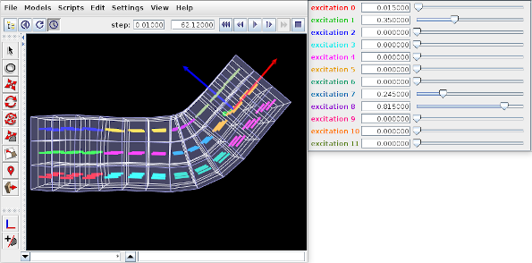
A simple example showing an FEM with material-based muscles is given by artisynth.demos.tutorial.ToyMuscleFem. It consists of a hex-element beam, with 12 muscles added in groups along its length, allowing it to flex in the x-z plane. A frame object is also attached to the right end. The code for the model, without the package and include directives, is listed below:
Within the build() method, the mech model is created in the usual way (lines 8-10). Gravity is turned off to give the muscles greater control over the FEM model’s configuration. The MechModel reference is stored in the class field myMech to enable any subclasses to have easy access to it; the same will be done for the FEM model and the attached frame.
The FEM model itself is created at lines (12-24). An instance of FemMuscleModel is created and then passed to FemFactory.createHexGrid(); this allows the model to be an instance of FemMuscleModel instead of FemModel3d. The model is assigned a linear material with Poisson’s ratio of 0 to allow it to be easily compressed. Muscle bundles will be material-based and will all use the same SimpleForceMuscle material that is assigned to the model’s muscleMaterial property. Density and damping parameters are defined so as to improve model stability when muscles are excited. Once the model is created, its left-hand nodes are fixed to provide anchoring (lines 27-32).
Muscle bundles are created at lines 36-58. There are 12 of them, arranged in three vertical layers and four horizontal sections. Each bundle is populated with 9 adjacent elements in the x-y plane. To find these elements, their center positions are calculated and then passed to the FEM method findNearestVolumetricElement(). The element is then added to the bundle with a resting activation direction parallel to the x axis. For visualization, each bundle’s line color is set to a distinct color from the numeric probe display palette, based on the bundle’s number (lines 53-54).
After the bundles have been added to the FEM model, a control is created to allow interactive control of their excitations (lines 88-95). Each widget is labeled excitation N, where N is the bundle number, and the label is colored to match the bundle’s line color. Finally, a frame is created and attached to the FEM model (lines 59-62), and render properties are set at lines 106-115: Muscle bundles are drawn by showing the activation direction in each element; the frame is displayed as a solid arrow with axis lengths of 0.3; the FEM line and face colors are set to blue-gray, and the surface is rendered and made transparent.
To run this example in ArtiSynth, select All demos > tutorial > ToyMuscleFem from the Models menu. Running the model and adjusting the exciters in the control panel will cause the FEM model to deform in various ways (Figure 1.15).
1.9.5 Example: comparison with two beam examples
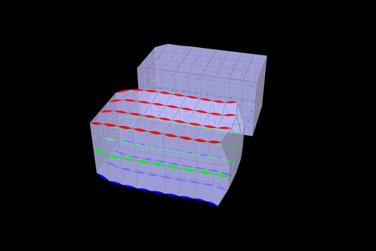
An example comparing a fibre-based and a material-based muscle is shown in Figure 1.16. The code can be found in artisynth.demos.tutorial.FemMuscleBeams. There are two FemMuscleModel beams in the model: one fibre-based, and one material-based. Each has three muscle bundles: one at the top (red), one in the middle (green), and one at the bottom (blue). In the figure, both muscles are fully activated. Note the deformed shape of the beams. In the fibre-based one, since forces only act between point on the fibres, the muscle seems to bulge. In the material-based muscle, the entire continuous volume contracts, leading to a uniform deformation.
Material-based muscles are more realistic. However, this often comes at the cost of stability. The added terms to the constitutive law are highly nonlinear, which may cause numerical issues as elements become highly contracted or highly deformed. Fibre-based muscles are, in general, more stable. However, they can lead to bulging and other deformation artifacts due to their discrete nature.
1.10 Material types
ArtiSynth FEM models support a variety of material types, including
linear, hyperelastic, and activated muscle materials, described in the
sections below. These can be used to supply the primary material for
either an entire FEM model or for specific elements (using the setMaterial() methods for either). They can also be used to supply
auxiliary materials, whose behavior is superimposed on the underlying
material, via either material bundles
(Section 1.8) or,
for FemMuscleModels, muscle bundles
(Section 1.9). Many of the properties for a given
material can be bound to a scalar or vector field
(Section LABEL:sec:femFields) to allow their values to vary across an
FEM model. In the descriptions below, properties for which this is
true will have a ![]() indicated under the “Field” entry in the
material’s property table.
indicated under the “Field” entry in the
material’s property table.
All materials are defined in the package artisynth.core.materials.
1.10.1 Linear
Linear materials determine Cauchy stress ![]() as a linear mapping
from the small deformation Cauchy strain
as a linear mapping
from the small deformation Cauchy strain ![]() ,
,
| (1.8) |
where ![]() is the elasticity tensor.
Both the stress and
strain are symmetric
is the elasticity tensor.
Both the stress and
strain are symmetric ![]() matrices,
matrices,
 |
(1.9) |
and can be expressed as 6-vectors using Voigt notation:
 |
(1.10) |
This allows the constitutive mapping to be expressed in matrix form as
| (1.11) |
where ![]() is the
is the ![]() elasticity matrix.
elasticity matrix.
Different Voigt notation mappings appear in the literature with regard to off-diagonal matrix entries. We use the one employed by FEBio [FEBioTheory2018]. Another common mapping is
Traditionally, Cauchy strain is computed from the symmetric part of
the deformation gradient ![]() using the formula
using the formula
| (1.12) |
where ![]() is the
is the ![]() identity matrix. However, ArtiSynth
materials support corotation, in which rotations are first
removed from
identity matrix. However, ArtiSynth
materials support corotation, in which rotations are first
removed from ![]() using a polar decomposition
using a polar decomposition
| (1.13) |
where ![]() is a (right-handed) rotation matrix and
is a (right-handed) rotation matrix and ![]() is symmetric
matrix.
is symmetric
matrix. ![]() is then used to compute the Cauchy strain:
is then used to compute the Cauchy strain:
| (1.14) |
Corotation is the default behavior for linear materials in ArtiSynth and allows models to handle large scale rotational deformations [ngan:fem:2008, muller2004interactive].
For linear materials, the stress/strain response is computed at a single integration point in the center of each element. This is done
to improve computational efficiency, as it allows the precomputation
of stiffness matrices that map nodal displacements onto nodal forces
for each element. This precomputed matrix can then be adjusted during
each simulation step to account for the rotation ![]() computed at each
element’s integration
point [ngan:fem:2008, muller2004interactive].
computed at each
element’s integration
point [ngan:fem:2008, muller2004interactive].
Specific linear material types are listed in the subsections below. All are subclasses of LinearMaterialBase, and in addition to their individual properties, all export a corotation property (default value true) that controls whether corotation is applied.
1.10.1.1 LinearMaterial
LinearMaterial is a standard isotropic linear material, which is also the default material for FEM models. Its elasticity matrix is given by
 |
(1.15) |
where the Lamé parameters ![]() and
and ![]() are
derived from Young’s modulus
are
derived from Young’s modulus ![]() and Poisson’s ratio
and Poisson’s ratio ![]() via
via
| (1.16) |
The material behavior is controlled by the following properties:
| Property | Description | Default | Field | |
|---|---|---|---|---|
| YoungsModulus | Young’s modulus | 500000 | ✓ | |
| PoissonsRatio | Poisson’s ratio | 0.33 | ||
| corotated | applies corotation if true | true |
LinearMaterials can be created with the following constructors:
| LinearMaterial() |
Create with default properties. |
| LinearMaterial (double E, double nu) |
Create with specified |
| LinearMaterial (double E, double nu, boolean corotated) |
Create with specified |
1.10.1.2 TransverseLinearMaterial
TransverseLinearMaterial
is a transversely isotropic linear material whose behavior is
symmetric about a prescribed polar axis. If the polar axis is
parallel to the ![]() axis, then the elasticity matrix is specified most
easily in terms of its inverse, or compliance matrix, according
to
axis, then the elasticity matrix is specified most
easily in terms of its inverse, or compliance matrix, according
to
 |
where ![]() and
and ![]() are Young’s moduli transverse
and parallel to the axis, respectively,
are Young’s moduli transverse
and parallel to the axis, respectively, ![]() and
and ![]() are
Poisson’s ratios transverse and parallel to the axis, and
are
Poisson’s ratios transverse and parallel to the axis, and ![]() is the
shear modulus.
is the
shear modulus.
The material behavior is controlled by the following properties:
| Property | Description | Default | Field | |
|---|---|---|---|---|
| youngsModulus | Young’s moduli transverse and parallel to the axis | ✓ | ||
| poissonsRatio | Poisson’s ratios transverse and parallel to the axis | |||
| shearModulus | shear modulus | 187970 | ✓ | |
| direction | direction of the polar axis | ✓ | ||
| corotated | applies corotation if true | true |
The youngsModulus and poissonsRatio properties are both described by Vector2d objects, while direction is described by a Vector3d. The direction property (as well as youngsModulus and shearModulus) can be bound to a field to allow its value to vary over an FEM model (Section LABEL:sec:femFields).
TransverseLinearMaterials can be created with the following constructors:
| TransverseLinearMaterial() |
Create with default properties. |
| TransverseLinearMaterial (Vector2d E, double G, Vector2d nu, boolean corotated) |
Create with specified |
1.10.1.3 AnisotropicLinearMaterial
AnisotropicLinearMaterial
is a general anisotropic linear material whose behavior is specified
by an arbitrary (symmetric) elasticity matrix ![]() .
The material behavior is controlled by the following properties:
.
The material behavior is controlled by the following properties:
| Property | Description | Default | Field | |
|---|---|---|---|---|
| stiffnessTensor | symmetric |
|||
| corotated | applies corotation if true | true |
The default value for stiffnessTensor is an isotropic elasticity
matrix corresponding to ![]() and
and ![]() .
.
AnisotropicLinearMaterials can be created with the following constructors:
| AnisotropicLinearMaterial() |
Create with default properties. |
| AnisotropicLinearMaterial (Matrix6dBase D) |
Create with specified elasticity |
| AnisotropicLinearMaterial (Matrix6dBase D, boolean corotated) |
Create with specified |
1.10.2 Hyperelastic materials
A hyperelastic material is defined by a strain energy density
function ![]() that is in general a function of the deformation gradient
that is in general a function of the deformation gradient
![]() , and more specifically a quantity derived from
, and more specifically a quantity derived from ![]() that is
rotationally invariant, such as the right Cauchy Green
tensor
that is
rotationally invariant, such as the right Cauchy Green
tensor ![]() , the left Cauchy Green
tensor
, the left Cauchy Green
tensor ![]() , or Green strain
, or Green strain
| (1.16) |
![]() is often described with respect to the first or second invariants
of these quantities, denoted by
is often described with respect to the first or second invariants
of these quantities, denoted by ![]() and
and ![]() and defined with
respect to a given matrix
and defined with
respect to a given matrix ![]() by
by
| (1.17) |
Alternatively, ![]() is sometimes defined with respect to the three
principal stretches of the deformation,
is sometimes defined with respect to the three
principal stretches of the deformation, ![]() , which are the eigenvalues of the symmetric component
, which are the eigenvalues of the symmetric component ![]() of the
polar decomposition of
of the
polar decomposition of ![]() in (1.13).
in (1.13).
If ![]() is expressed with respect to
is expressed with respect to ![]() , then the second
Piola-Kirchhoff stress
, then the second
Piola-Kirchhoff stress ![]() is given by
is given by
| (1.18) |
from which the Cauchy stress can be obtained via
| (1.19) |
Many of the hyperelastic materials described below are incompressible, in the sense that ![]() is partitioned into a deviatoric component that is volume invariant and a dilational
component that depends solely on volume changes.
Volume change is
characterized by
is partitioned into a deviatoric component that is volume invariant and a dilational
component that depends solely on volume changes.
Volume change is
characterized by ![]() , with the change in volume given by
, with the change in volume given by ![]() and
and ![]() indicating no volume change. Deviatoric
changes are characterized by
indicating no volume change. Deviatoric
changes are characterized by ![]() , with
, with
| (1.20) |
and so the partitioned strain energy density function assumes the form
| (1.21) |
where the ![]() term is the deviatoric contribution and
term is the deviatoric contribution and
![]() is the volumetric potential that enforces incompressibility.
is the volumetric potential that enforces incompressibility.
![]() may also be expressed with respect to the right deviatoric
Cauchy Green tensor
may also be expressed with respect to the right deviatoric
Cauchy Green tensor ![]() or the left deviatoric Cauchy Green
tensor
or the left deviatoric Cauchy Green
tensor ![]() , respectively defined by
, respectively defined by
| (1.22) |
ArtiSynth supplies different forms of ![]() , as specified by a
material’s bulkPotential property and detailed in
Section 1.7.3. All of the available potentials depend
on a bulkModulus property
, as specified by a
material’s bulkPotential property and detailed in
Section 1.7.3. All of the available potentials depend
on a bulkModulus property ![]() , and so
, and so ![]() is often
expressed as
is often
expressed as ![]() . A larger bulk modulus will make the
material more incompressible, with effective incompressibility
typically achieved by setting
. A larger bulk modulus will make the
material more incompressible, with effective incompressibility
typically achieved by setting ![]() to a value that exceeds the
other elastic moduli in the material by a factor of 100 or more.
All incompressible materials are subclasses of
IncompressibleMaterialBase.
to a value that exceeds the
other elastic moduli in the material by a factor of 100 or more.
All incompressible materials are subclasses of
IncompressibleMaterialBase.
1.10.2.1 St Venant-Kirchoff material
StVenantKirchoffMaterial
is a compressible isotropic material that extends isotropic linear
elasticity to large deformations.
The strain energy density is most easily expressed as a function
of the Green strain ![]() :
:
| (1.23) |
where the Lamé parameters ![]() and
and ![]() are
derived from Young’s modulus
are
derived from Young’s modulus ![]() and Poisson’s ratio
and Poisson’s ratio ![]() according to (1.16).
From this definition it follows that the second Piola-Kirchoff stress
tensor is given by
according to (1.16).
From this definition it follows that the second Piola-Kirchoff stress
tensor is given by
| (1.24) |
The material behavior is controlled by the following properties:
| Property | Description | Default | Field | |
|---|---|---|---|---|
| YoungsModulus | Young’s modulus | 500000 | ✓ | |
| PoissonsRatio | Poisson’s ratio | 0.33 |
StVenantKirchoffMaterials can be created with the following constructors:
| StVenantKirchoffMaterial() |
Create with default properties. |
| StVenantKirchoffMaterial (double E, double nu) |
Create with specified elasticity |
1.10.2.2 Neo-Hookean material
NeoHookeanMaterial
is a compressible isotropic material with a strain energy density
expressed as a function of the first invariant ![]() of the right
Cauchy-Green tensor
of the right
Cauchy-Green tensor ![]() and
and ![]() :
:
| (1.24) |
where the Lamé parameters ![]() and
and ![]() are derived from
Young’s modulus
are derived from
Young’s modulus ![]() and Poisson’s ratio
and Poisson’s ratio ![]() via
(1.16). The Cauchy stress can be expressed in terms of
the left Cauchy-Green tensor
via
(1.16). The Cauchy stress can be expressed in terms of
the left Cauchy-Green tensor ![]() as
as
| (1.25) |
The material behavior is controlled by the following properties:
| Property | Description | Default | Field | |
|---|---|---|---|---|
| YoungsModulus | Young’s modulus | 500000 | ✓ | |
| PoissonsRatio | Poisson’s ratio | 0.33 |
NeoHookeanMaterials can be created with the following constructors:
| NeoHookeanMaterial() |
Create with default properties. |
| NeoHookeanMaterial (double E, double nu) |
Create with specified elasticity |
1.10.2.3 Incompressible neo-Hookean material
IncompNeoHookeanMaterial
is an incompressible version of the neo-Hookean material,
with a strain energy density expressed in terms of the
first invariant ![]() of the deviatoric
right Cauchy-Green tensor
of the deviatoric
right Cauchy-Green tensor ![]() , plus a potential
function
, plus a potential
function ![]() to enforce incompressibility:
to enforce incompressibility:
| (1.25) |
The material behavior is controlled by the following properties:
| Property | Description | Default | Field | |
|---|---|---|---|---|
| shearModulus | shear modulus | 150000 | ✓ | |
| bulkModulus | bulk modulus for incompressibility | 100000 | ✓ | |
| bulkPotential | incompressibility potential function |
QUADRATIC |
IncompNeoHookeanMaterials can be created with the following constructors:
| IncompNeoHookeanMaterial() |
Create with default properties. |
| IncompNeoHookeanMaterial (double G, double kappa) |
Create with specified elasticity |
1.10.2.4 Mooney-Rivlin material
MooneyRivlinMaterial
is an incompressible isotropic material with a strain energy density
expressed as a polynomial of the first and second invariants ![]() and
and ![]() of the right deviatoric Cauchy-Green
tensor
of the right deviatoric Cauchy-Green
tensor ![]() . ArtiSynth supplies a five parameter version of this
model, with a strain energy density given by
. ArtiSynth supplies a five parameter version of this
model, with a strain energy density given by
| (1.25) |
A two-parameter version (![]() ,
, ![]() ) is often found in the
literature, consisting of only the first two terms:
) is often found in the
literature, consisting of only the first two terms:
| (1.26) |
The material behavior is controlled by the following properties:
| Property | Description | Default | Field | |
|---|---|---|---|---|
| C10 | first coefficient | 150000 | ✓ | |
| C01 | second coefficient | 0 | ✓ | |
| C11 | third coefficient | 0 | ✓ | |
| C20 | fourth coefficient | 0 | ✓ | |
| C02 | fifth coefficient | 0 | ✓ | |
| bulkModulus | bulk modulus for incompressibility | 100000 | ✓ | |
| bulkPotential | incompressibility potential function |
QUADRATIC |
MooneyRivlinMaterials can be created with the following constructors:
| MooneyRivlinMaterial() |
Create with default properties. |
| MooneyRivlinMaterial (double C10, double C01, double C11, double C20, double C02, double kappa) |
Create with specified coefficients. |
1.10.2.5 Ogden material
OgdenMaterial
is an incompressible material with a strain energy density
expressed as a function of the deviatoric principal stretches ![]() :
:
 |
(1.26) |
ArtiSynth allows a maximum of six terms, corresponding to ![]() , and
the material behavior is controlled by the following properties:
, and
the material behavior is controlled by the following properties:
| Property | Description | Default | Field | |
|---|---|---|---|---|
| Mu1 | first multiplier | 300000 | ✓ | |
| Mu2 | second multiplier | 0 | ✓ | |
| ... | ... | ... | 0 | ✓ |
| Mu6 | final multiplier | 0 | ✓ | |
| Alpha1 | first multiplier | 2 | ✓ | |
| Alpha2 | second multiplier | 2 | ✓ | |
| ... | ... | ... | 2 | ✓ |
| Alpha6 | final multiplier | 2 | ✓ | |
| bulkModulus | bulk modulus for incompressibility | 100000 | ✓ | |
| bulkPotential | incompressibility potential function |
QUADRATIC |
OgdenMaterials can be created with the following constructors:
| OgdenMaterial() |
Create with default properties. |
| OgdenMaterial (double[] mu, double[] alpha, double kappa) |
Create with specified |
1.10.2.6 Fung orthotropic material
FungOrthotropicMaterial
is an incompressible orthotropic material defined with respect to an
![]() -
-![]() -
-![]() coordinate system expressed by a
coordinate system expressed by a ![]() rotation
matrix
rotation
matrix ![]() . The strain energy density is expressed as a function of
the deviatoric Green strain
. The strain energy density is expressed as a function of
the deviatoric Green strain
| (1.26) |
and the three unit direction vectors ![]() representing the columns of
representing the columns of ![]() . Letting
. Letting ![]() and defining
and defining
| (1.27) |
the energy density is given by
 |
(1.28) |
where ![]() is a material coefficient and
is a material coefficient and ![]() and
and ![]() are
the orthotropic Lamé parameters.
are
the orthotropic Lamé parameters.
At present, the coordinate frame ![]() is not defined in the material,
but can be specified on a per-element basis using the element method
setFrame(Matrix3dBase). For example:
is not defined in the material,
but can be specified on a per-element basis using the element method
setFrame(Matrix3dBase). For example:
One should be careful to ensure that the argument to setFrame() is in fact an orthogonal rotation matrix as this will not be otherwise enforced.
The material behavior is controlled by the following properties:
| Property | Description | Default | Field | |
|---|---|---|---|---|
| mu1 | second Lamé parameter along |
1000 | ✓ | |
| mu2 | second Lamé parameter along |
1000 | ✓ | |
| mu3 | second Lamé parameter along |
1000 | ✓ | |
| lam11 | first Lamé parameter along |
2000 | ✓ | |
| lam22 | first Lamé parameter along |
2000 | ✓ | |
| lam33 | first Lamé parameter along |
2000 | ✓ | |
| lam12 | first Lamé parameter for |
2000 | ✓ | |
| lam23 | first Lamé parameter for |
2000 | ✓ | |
| lam31 | first Lamé parameter for |
2000 | ✓ | |
| C | C coefficient | 1500 | ✓ | |
| bulkModulus | bulk modulus for incompressibility | 100000 | ✓ | |
| bulkPotential | incompressibility potential function |
QUADRATIC |
FungOrthotropicMaterials can be created with the following constructors:
| FungOrthotropicMaterial() |
Create with default properties. |
| FungOrthotropicMaterial (double mu1, double mu2, double mu3, double lam11, double lam22, double lam33, double lam12, double lam23, double lam31, double C, double kappa) |
Create with specified properties. |
1.10.2.7 Yeoh material
YeohMaterial is an incompressible isotropic material that implements a Yeoh model with a strain energy density containing up to five terms:
 |
(1.28) |
where ![]() is the first invariant of the right deviatoric Cauchy Green
tensor and
is the first invariant of the right deviatoric Cauchy Green
tensor and ![]() are the material coefficients.
The material behavior is controlled by the following properties:
are the material coefficients.
The material behavior is controlled by the following properties:
| Property | Description | Default | Field | |
|---|---|---|---|---|
| C1 | first coefficient (shear modulus) | 150000 | ✓ | |
| C2 | second coefficient | 0 | ✓ | |
| C3 | third coefficient | 0 | ✓ | |
| C4 | fourth coefficient | 0 | ✓ | |
| C5 | fifth coefficient | 0 | ✓ | |
| bulkModulus | bulk modulus for incompressibility | 100000 | ✓ | |
| bulkPotential | incompressibility potential function |
QUADRATIC |
YeohMaterials can be created with the following constructors:
| YeohMaterial() |
Create with default properties. |
| YeohMaterial (double C1, double C2, double C3, double kappa) |
Create three term material with |
| YeohMaterial (double C1, double C2, double C3, double C4, double C5, double kappa) |
Create five term material with |
1.10.2.8 Arruda-Boyce material
ArrudaBoyceMaterial is an incompressible isotropic material that implements the Arruda-Boyce model [arruda1993three]. Its strain energy density is given by
 |
(1.28) |
where ![]() is the initial modulus,
is the initial modulus, ![]() the
locking stretch,
the
locking stretch, ![]() the first invariant of the
right deviatoric Cauchy Green tensor, and
the first invariant of the
right deviatoric Cauchy Green tensor, and
 |
The material behavior is controlled by the following properties:
| Property | Description | Default | Field | |
|---|---|---|---|---|
| mu | initial modulus | 1000 | ✓ | |
| lambdaMax | locking stretch | 2.0 | ✓ | |
| bulkModulus | bulk modulus for incompressibility | 100000 | ✓ | |
| bulkPotential | incompressibility potential function |
QUADRATIC |
ArrudaBoyceMaterials can be created with the following constructors:
| ArrudaBoyceMaterial() |
Create with default properties. |
| ArrudaBoyceMaterial (double mu, double lmax, double kappa) |
Create with specified |
1.10.2.9 Veronda-Westmann material
VerondaWestmannMaterial is an incompressible isotropic material that implements the Veronda-Westmann model [veronda1970mechanical]. Its strain energy density is given by
| (1.29) |
where ![]() and
and ![]() are material coefficients and
are material coefficients and ![]() and
and
![]() the first and second invariants of the right deviatoric
Cauchy Green tensor.
the first and second invariants of the right deviatoric
Cauchy Green tensor.
The material behavior is controlled by the following properties:
| Property | Description | Default | Field | |
|---|---|---|---|---|
| C1 | first coefficient | 1000 | ✓ | |
| C2 | second coefficient | 10 | ✓ | |
| bulkModulus | bulk modulus for incompressibility | 100000 | ✓ | |
| bulkPotential | incompressibility potential function |
QUADRATIC |
VerondaWestmannMaterials can be created with the following constructors:
| VerondaWestmannMaterial() |
Create with default properties. |
| VerondaWestmannMaterial (double C1, double C2, double kappa) |
Create with specified |
1.10.2.10 Incompressible material
IncompressibleMaterial is an incompressible isotropic material that implements pure incompressibility, with an energy density function given by
| (1.29) |
Because it responds only to dilational strains, it must be used in conjunction with another material to resist deviatoric strains. In this context, it can be used to provide dilational support to deviatoric-only materials such as the FullBlemkerMuscle (Section 1.10.3.3).
The material behavior is controlled by the following properties:
| Property | Description | Default | Field | |
|---|---|---|---|---|
| bulkModulus | bulk modulus for incompressibility | 100000 | ✓ | |
| bulkPotential | incompressibility potential function |
QUADRATIC |
IncompressibleMaterials can be created with the following constructors:
| IncompressibleMaterial() |
Create with default values. |
| IncompressibleMaterial (double kappa) |
Create with specified |
1.10.3 Muscle materials
Muscle materials are used to exert stress along a particular direction within a material. This stress may contain both an active component, which depends on the muscle excitation, and a passive component, which depends solely on the stretch along the prescribed direction. Because most muscle materials act only along one direction, they are typically deployed within an FEM as additional materials that act in addition to an underlying material. This can be done using either muscle bundles within a FemMuscleModel (Section 1.9.1.1) or material bundles within any FEM model (Sections 1.8 and LABEL:RadialMuscle:sec).
All of the muscle materials described below assume (near)
incompressibility, and so the directional stress is a function of the
deviatoric stretch ![]() along the muscle direction instead of the
overall stretch
along the muscle direction instead of the
overall stretch ![]() . The former can be determined from the
latter via
. The former can be determined from the
latter via
| (1.29) |
where ![]() is the determinant of the deformation gradient. The
directional Cauchy stress
is the determinant of the deformation gradient. The
directional Cauchy stress ![]() resulting from the material is
computed from
resulting from the material is
computed from
 |
(1.30) |
where ![]() is a force term,
is a force term, ![]() is a unit vector indicating
the current muscle direction in spatial coordinates, and
is a unit vector indicating
the current muscle direction in spatial coordinates, and ![]() is the
is the ![]() identity matrix. In a purely passive case when the force arises
from a stress energy density function
identity matrix. In a purely passive case when the force arises
from a stress energy density function ![]() , we have
, we have
| (1.31) |
The muscle direction is specified in one of two ways, depending on how
the muscle material is deployed. All muscle materials export a
property restDir which specifies the direction in material
(rest) coordinates. It has a default value of ![]() , and can
be either set explicitly or bound to a field to allow it to vary over the
entire model (Section LABEL:RadialMuscle:sec). However, if a muscle
material is deployed within a muscle bundle
(Section 1.9.1), then the restDir property is
ignored and the direction is instead specified by the
MuscleElementDesc components contained
within the bundle (Section 1.9.3).
, and can
be either set explicitly or bound to a field to allow it to vary over the
entire model (Section LABEL:RadialMuscle:sec). However, if a muscle
material is deployed within a muscle bundle
(Section 1.9.1), then the restDir property is
ignored and the direction is instead specified by the
MuscleElementDesc components contained
within the bundle (Section 1.9.3).
Likewise, muscle excitation is specified using the material’s excitation property, unless the material is deployed within a muscle bundle, in which case it is controlled by the excitation property of the bundle.
1.10.3.1 Generic muscle
GenericMuscle
is a muscle material whose force term ![]() is given by
is given by
| (1.32) |
where ![]() is the excitation signal,
is the excitation signal, ![]() is a maximum stress
term, and
is a maximum stress
term, and ![]() is a passive force given by
is a passive force given by
 |
(1.33) |
In the equation above, ![]() is the exponential stress coefficient,
is the exponential stress coefficient,
![]() is the uncrimping factor, and
is the uncrimping factor, and ![]() and
and ![]() are computed to
provide
are computed to
provide ![]() continuity at
continuity at ![]() .
.
The material behavior is controlled by the following properties:
| Property | Description | Default | Field | |
|---|---|---|---|---|
| maxStress | maximum stress | 30000 | ✓ | |
| maxLambda |
|
1.4 | ✓ | |
| expStressCoeff | exponential stress coefficient | 0.05 | ✓ | |
| uncrimpingFactor | uncrimping factor | 6.6 | ✓ | |
| restDir | direction in material coordinates | ✓ | ||
| excitation | activation signal | 0 |
GenericMuscles can be created with the following constructors:
| GenericMuscle() |
Create with default values. |
| GenericMuscle (double maxLambda, double maxStress, double expStressCoef, double uncrimpFactor) |
Create with specified |
The constructors do not specify restDir. If the material is not being deployed within a muscle bundle, then restDir should also be set appropriately, either directly or via a field (Section LABEL:RadialMuscle:sec).
1.10.3.2 Blemker muscle
BlemkerMuscle
is a muscle material implementing the directional component of the
model proposed by Sylvia Blemker [blemker:2005:muscle]. Its force
term ![]() is given by
is given by
| (1.33) |
where ![]() is a maximum stress term,
is a maximum stress term, ![]() is the excitation
signal,
is the excitation
signal, ![]() is an active force-length curve, and
is an active force-length curve, and ![]() is
the passive force.
is
the passive force. ![]() and
and ![]() are described in
terms of
are described in
terms of ![]() :
:
 |
(1.34) |
and
 |
(1.35) |
In the equation for ![]() ,
, ![]() is the exponential stress
coefficient,
is the exponential stress
coefficient, ![]() is the uncrimping factor, and
is the uncrimping factor, and ![]() and
and ![]() are
computed to provide
are
computed to provide ![]() continuity at
continuity at ![]() .
.
The material behavior is controlled by the following properties:
| Property | Description | Default | Field | |
|---|---|---|---|---|
| maxStress | maximum stress | 300000 | ✓ | |
| optLambda |
|
1 | ✓ | |
| maxLambda |
|
1.4 | ✓ | |
| expStressCoeff | exponential stress coefficient | 0.05 | ✓ | |
| uncrimpingFactor | uncrimping factor | 6.6 | ✓ | |
| restDir | direction in material coordinates | ✓ | ||
| excitation | activation signal | 0 |
BlemkerMuscles can be created with the following constructors:
| BlemkerMuscle() |
Create with default values. |
| BlemkerMuscle (double maxLam, double optLam, double maxStress, double expStressCoef, double uncrimpFactor) |
Create with specified |
The constructors do not specify restDir. If the material is not being deployed within a muscle bundle, then restDir should also be set appropriately, either directly or via a field (Section LABEL:RadialMuscle:sec).
1.10.3.3 Full Blemker muscle
FullBlemkerMuscle
is a muscle material implementing the entire model proposed by Sylvia
Blemker [blemker:2005:muscle]. This includes the directional
stress described in Section 1.10.3.2, plus additional
passive terms to model the tissue material matrix. The latter is based
on a strain energy density function ![]() given by
given by
| (1.35) |
where ![]() and
and ![]() are the along-fibre and cross-fibre
shear moduli, respectively, and
are the along-fibre and cross-fibre
shear moduli, respectively, and ![]() and
and ![]() are
Criscione invariants. The latter are defined as follows: Let
are
Criscione invariants. The latter are defined as follows: Let ![]() and
and ![]() be the invariants of the deviatoric left Cauchy
Green tensor
be the invariants of the deviatoric left Cauchy
Green tensor ![]() ,
, ![]() the unit vector giving the current muscle
direction in spatial coordinates, and
the unit vector giving the current muscle
direction in spatial coordinates, and ![]() and
and ![]() additional invariants defined by
additional invariants defined by
| (1.36) |
Then, defining
 |
![]() and
and ![]() are given by
are given by
 |
(1.37) | |||
 |
(1.38) |
At present, FullBlemkerMuscle does not implement a volumetric potential function
. That means it responds solely to deviatoric strains, and so if it is being used as a model’s primary material, it should be augmented with an additional material to provide resistance to compression. A simple choice for this is the purely incompressible material IncompressibleMaterial, described in Section 1.10.2.10.
The material behavior is controlled by the following properties:
| Property | Description | Default | Field | |
|---|---|---|---|---|
| maxStress | maximum stress | 300000 | ✓ | |
| optLambda |
|
1 | ✓ | |
| maxLambda |
|
1.4 | ✓ | |
| expStressCoeff | exponential stress coefficient | 0.05 | ✓ | |
| uncrimpingFactor | uncrimping factor | 6.6 | ✓ | |
| G1 | along-fibre shear modulus | 0 | ✓ | |
| G2 | cross-fibre shear modulus | 0 | ✓ | |
| restDir | direction in material coordinates | ✓ | ||
| excitation | activation signal | 0 |
FullBlemkerMuscles can be created with the following constructors:
| FullBlemkerMuscle() |
Create with default values. |
| BlemkerMuscle (double maxLam, double optLam, double maxStress, double expStressCoef, double uncrimpFactor, double G1, double G2) |
Create with |
The constructors do not specify restDir. If the material is not being deployed within a muscle bundle, then restDir should also be set appropriately, either directly or via a field (Section LABEL:RadialMuscle:sec).
1.10.3.4 Simple force muscle
SimpleForceMuscle
is a very simple muscle material whose force term ![]() is
given by
is
given by
| (1.39) |
where ![]() is the excitation signal and
is the excitation signal and ![]() is a maximum
stress term. It can be useful as a debugging tool.
is a maximum
stress term. It can be useful as a debugging tool.
The material behavior is controlled by the following properties:
| Property | Description | Default | Field | |
|---|---|---|---|---|
| maxStress | maximum stress | 30000 | ✓ | |
| restDir | direction in material coordinates | ✓ | ||
| excitation | activation signal | 0 |
SimpleForceMuscles can be created with the following constructors:
| SimpleForceMuscle() |
Create with default values. |
| SimpleForceMuscle (double maxStress) |
Create with specified |
The constructors do not specify restDir. If the material is not being deployed within a muscle bundle, then restDir should also be set appropriately, either directly or via a field (Section LABEL:RadialMuscle:sec).
1.11 Stress, strain and strain energy
An ArtiSynth FEM model has the capability to compute a variety of stress and strain measures at each of its nodes, as well as strain energy for each element and for the entire model.
1.11.1 Computing nodal values
Stress, strain, and strain energy density can be computed at each node of an FEM model. By default, these quantities are not computed, in order to conserve computing power. However, their computation can be enabled with the FemModel3d properties computeNodalStress, computeNodalStrain and computeNodalEnergyDensity, which can be set either in the GUI, or using the following accessor methods:
| void setComputeNodalStress(boolean) |
Enable stress to be computed at each node. |
| boolean getComputeNodalStress() |
Queries if nodal stress computation enabled. |
| void setComputeNodalStrain(boolean) |
Enable strain to be computed at each node. |
| boolean getComputeNodalStrain() |
Queries if nodal strain computation enabled. |
| void setComputeNodalEnergyDensity(boolean) |
Enable strain energy density to be computed at each node. |
| boolean getComputeNodalEnergyDensity() |
Queries if nodal strain energy density computation enabled. |
Setting these properties to true will cause their respective values to be computed at the nodes during each subsequent simulation step. This is done by computing values at the element integration points, extrapolating these values to the nodes, and then averaging them across the contributions from all surrounding elements.
Once computed, the values may be obtained at each node using the following FemNode3d methods:
| SymmetricMatrix3d getStress() |
Returns the current Cauchy stress at the node. |
| SymmetricMatrix3d getStrain() |
Returns the current strain at the node. |
| double getEnergyStrain() |
Returns the current strain energy density at the node. |
The stress value is the Cauchy stress. The strain values depend on the
primary material within each element: if the material is linear,
strain will be the small deformation Cauchy strain (co-rotated if the
material’s corotated property is true), while otherwise it
will be Green strain ![]() :
:
| (1.39) |
where ![]() is the right Cauchy-Green tensor.
is the right Cauchy-Green tensor.
1.11.2 Scalar stress/strain measures
Stress or strain values are tensor quantities represented by symmetric
![]() matrices. If they are being computed at the nodes, a
variety of scalar quantities can be extracted from them, using the
FemNode3d method
matrices. If they are being computed at the nodes, a
variety of scalar quantities can be extracted from them, using the
FemNode3d method
| double getStressStrainMeasure(StressStrainMeasure m) |
where StressStrainMeasure is an enumerated type with the following entries:
- VonMisesStress
-
von Mises stress, equal to

where
 the second invariant of the average deviatoric stress.
 - MAPStress
-
Absolute value of the maximum principle Cauchy stress.
- MaxShearStress
-
Maximum shear stress, given by

where
 ,
, 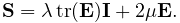 and
and  are the eigenvalues of the stress tensor.
 - VonMisesStrain
-
von Mises strain, equal to

where
the second invariant of the average deviatoric strain. - MAPStrain
-
Absolute value of the maximum principle strain.
- MaxShearStrain
-
Maximum shear strain, given by
where
, and are the eigenvalues of the strain tensor. - EnergyDensity
-
Strain energy density.
These quantities can also be queried with the following convenience methods:
| double getVonMisesStress() |
Return the von Mises stress. |
| double getMAPStress() |
Return the maximum absolute principle stress. |
| double getMaxShearStress() |
Return the maximum shear stress. |
| double getVonMisesStrain() |
Return the von Mises strain. |
| double getMAPStrain() |
Return the maximum absolute principle strain. |
| double getMaxShearStrain() |
Return the maximum shear strain. |
| double getEnergyDensity() |
Return the strain energy density. |
For muscle-activated FEM materials, strain energy density is currently computed only for the passive portions of the material; no energy density is computed for the stress component that depends on muscle activation.
As indicated above, extracting these measures requires that the appropriate underling quantity (stress, strain or strain energy density) is being computed at the nodes; otherwise, 0 will be returned. To ensure that the appropriate underlying quantity is being computed for a specific measure, one may use the FemModel3d method
| void setComputeNodalStressStrain (StressStrainMeasure m) |
1.11.3 Strain energy
Strain energy density can be integrated over an FEM model’s volume to compute a total strain energy. Again, to save computational resources, this must be explicitly enabled using the FemModel3d property computeStrainEnergy, which can be set either in the GU or using the accessor methods:
| void setComputeStrainEnergy(boolean) |
Enable strain energy computation. |
| boolean getComputeStrainEnergy() |
Queries strain energy computation. |
Once computation is enabled, strain energy is exported for the entire model using the read-only strainEnergy property, which can be accessed using
| double getStrainEnergy() |
The FemElement method getStrainEnergy() returns the strain energy for individual elements.
1.12 Rendering and Visualizations
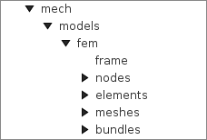
An ArtiSynth FEM model can be rendered in a wide variety of ways, by adjusting the rendering of its nodes, elements, meshes (including the surface and other embedded meshes), and, for FemMuscleModel, muscle bundles. Properties for controlling the rendering include both the standard RenderProps (Section LABEL:RenderProperties:sec) as well as more specific properties. These can be set either in code, as described below, or by selecting the desired components (or their lists) and then choosing either Edit render props ... (for standard render properties) or Edit properties ... (for component-specific render properties) from the context menu. As mentioned in Section LABEL:RenderProperties:sec, standard render properties are inherited, and so if not explicitly specified within a given component, will assume whatever value has been set in the nearest ancestor component, or their default value. Some component-specific render properties are inherited as well.
One very direct way to control the rendering is to control the visibility of the various component lists. This can be done by selecting them in the navigation panel (Figure 1.17) and then choosing “Set invisible” or “Set visible”, as appropriate. It can also be done in code, as shown in the fragment below making the elements and nodes of an FEM model invisible:
1.12.1 Nodes
Node rendering is controlled by the point render properties of the standard RenderProps. By default, nodes are set to render as gray points one pixel wide, and so are not highly visible. To increase their visibility, and make them easier to select in the viewer, one can make them appear as spheres of a specified radius and color. In code, this can be done using the RenderProps.setSphericalPoints() method, as in this example,
which sets the default rendering for all points within the FEM model (which includes the nodes) to be green spheres of radius 0.01. To restrict this to the node list specifically, one could supply fem.getNodes() instead of fem to setSphericalPoints().
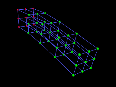
It is also possible to set render properties for individual nodes. For instance, one may wish to mark nodes that are non-dynamic using a different color:
Figure 1.18 shows an FEM model with nodes rendered as spheres, with the dynamic nodes colored green and the non-dynamic ones red.
1.12.2 Elements
By default, elements are rendered as wireframe outlines, using the lineColor and lineWidth properties of the standard render properties, with defaults of “gray” and 1. To improve visibility, one may wish the change the line color or size, as illustrated by the following fragment:
This will set the default line color and width for all components within the FEM model. To restrict this to the elements only, one can specify fem.getElements() (and/or fem.getShellElements()) to the set methods. The fragment above is illustrated in Figure 1.19 (left) for a model created with a call to FemFactory.createHexTorus().
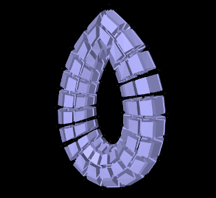
|
Elements can also be rendered as widgets that depict an approximation
of their shape displayed at some fraction of the element’s size (this
shape will be 3D for volumetric elements and 2D for shell
elements). This is controlled using the FemModel3d property elementWidgetSize, which is restricted to the range ![]() and
describes the size of the widgets relative to the element size. If
elementWidgetSize is 0 then no widgets are displayed. The
widget color is controlled using the faceColor and alpha
properties of the standard render properties. The following code
fragment enables element widget rendering for an FEM model, as
illustrated in Figure 1.19 (right):
and
describes the size of the widgets relative to the element size. If
elementWidgetSize is 0 then no widgets are displayed. The
widget color is controlled using the faceColor and alpha
properties of the standard render properties. The following code
fragment enables element widget rendering for an FEM model, as
illustrated in Figure 1.19 (right):
Since setting faceColor for the whole FEM model will also set the default face color for its meshes, one may wish to restrict setting this to the elements only, by specifying fem.getElements() and/or fem.getShellElements() to setFaceColor().
Element widgets can provide a easy way to select specific elements. The elementWidgetSize property is also present as an inherited property in the volumetric and shell element lists (elements and shellElements), as well as individual elements, and so widget rendering can be controlled on a per-element basis.
1.12.3 Surface and other meshes
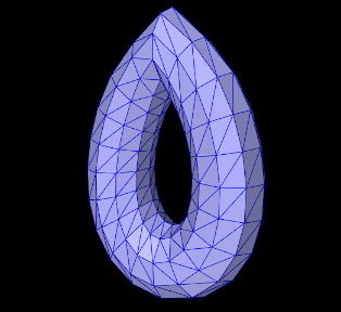
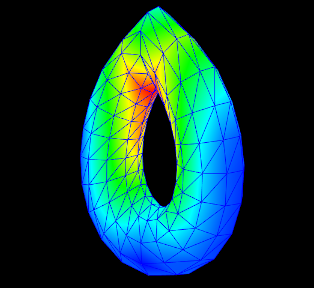
|
A FEM model can also be rendered using its surface mesh and/or other mesh geometry (Section 1.19). How meshes are rendered is controlled by the property surfaceRendering, which can be assigned any of the values shown in Table 1.5. The value None causes nothing to be rendered, while Shaded causes a mesh to be rendered using the standard rendering properties appropriate to that mesh. For polygonal meshes (which include the surface mesh), this will be done according to the face rendering properties in same way as for rigid bodies (Section LABEL:rigidBodyRendering:sec). These properties include faceColor, shading, alpha, faceStyle, drawEdges, edgeWidth, and edgeColor (or lineColor if the former is not set). The following code fragment sets an FEM surface to be rendered with blue-gray faces and dark blue edges (Figure 1.20, left):
| Value | Description |
|---|---|
| None | mesh is not rendered |
| Shaded | rendered as a mesh using the standard rendering properties |
| Stress | color map of the von Mises stress |
| Strain | color map the von Mises strain |
| MAPStress | color map of the maximum absolute value principal stress |
| MAPStrain | color map of the maximum absolute value principal strain |
| MaxShearStress | color map of the maximum shear stress |
| MaxStearStrain | color map of the maximum sheer strain |
| EnergyDensity | color map of the strain energy density |
Other values of surfaceRendering cause polygonal meshes to be displayed as a color map showing the various stress or strain measures shown in Table 1.5 and described in greater detail in Section 1.11.2. The fragment below sets an FEM surface to be rendered to show the von Mises stress (Figure 1.20, right), while also rendering the edges as dark blue:
The color maps used in stress/strain rendering are controlled using the following additional properties:
- stressPlotRange
-
The range of numeric values associated with the color map. These are either fixed or updated automatically, according to the property stressPlotRanging. Values outside the range are truncated.
- stressPlotRanging
-
Describes if and how stressPlotRange is updated:
- Fixed
-
Range does not change and should be set by the application.
- Auto
-
Range automatically expands to contain the most recently computed values. Note that this does not cause the range to contract.
- colorMap
-
Value is a delegate object that converts stress and strain values to colors. Various types of maps exist, including HueColorMap (the default), GreyscaleColorMap, RainbowColorMap, and JetColorMap. These all implement the ColorMap interface.
All of these properties are inherited and exported both by FemModel3d and the individual mesh components (which are instances of FemMeshComp), allowing mesh rendering to be controlled on a per-mesh basis.
1.12.4 FEM-based muscles
FemMuscleModel and its subcomponents MuscleBundle export additional properties to control the rendering of muscle bundles and their associated fibre directions. These include:
- directionRenderLen
-
A scalar in the range
![[0,1]](mi/mi968.png) , which if
, which if  causes the fibre
directions to be rendered within the elements associated with a MuscleBundle (Section 1.9.3). The directions
are rendered as line segments, controlled by the standard line
render properties lineColor and lineWidth, and the value
of directionRenderLen specifies the length of this segment
relative to the size of the element.
causes the fibre
directions to be rendered within the elements associated with a MuscleBundle (Section 1.9.3). The directions
are rendered as line segments, controlled by the standard line
render properties lineColor and lineWidth, and the value
of directionRenderLen specifies the length of this segment
relative to the size of the element. - directionRenderType
-
If directionRenderLen
, this property specifics where the fibre directions should be rendered within muscle bundle
elements. The value ELEMENT causes a single direction to be
rendered at the element center, while INTEGRATION_POINTS causes
directions to be rendered at each of the element’s integration points. - elementWidgetSize
-
A scalar in the range
, which if causes the elements
within a muscle bundle to be rendered using an element widget (Section
1.12.2).
Since these properties are inherited and exported by both FemMuscleModel and MuscleBundle, they can be set for the FEM muscle model as a whole or for individual muscle bundles.
The code fragment below sets the element fibre directions for two muscle bundles to be drawn, one in red and one in green, using a directionRenderLen of 0.5. Each bundle runs horizontally along an FEM beam, one at the top and the other at the bottom (Figure 1.21, left):
By default, directionRenderType is set to ELEMENT and so directions are drawn at the element centers. Setting directionRenderType to INTEGRATION_POINT causes the directions to be drawn at each integration points (Figure 1.21, right), which is useful when directions are specified at integration points (Section 1.9.3).
If we are only interested in seeing the elements associated with a muscle bundle, we can use its elementWidgetSize property to draw the elements as widgets (Figure 1.22, left). For this, the last two lines of the fragment above could be replaced with
Finally, if the muscle bundle contains point-to-point fibres (Section 1.9.2), these can be rendered by setting the line properties of the standard render properties. For example, the fibre rendering of Figure 1.22 (right) can be set up using the code
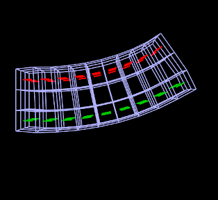

|
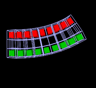

|
1.12.5 Color bars
To display values corresponding to colors, a ColorBar needs to be added to the RootModel. Color bars are general Renderable objects that are only used for visualizations. They are added to the display using the
method in RootModel. Color bars also have a ColorMap associated with it. The following functions are useful for controlling its visualization:
The normalized location specifies sizes relative to the screen size (1 = screen width/height). The location override, if values are non-zero, will override the normalized location, specifying values in absolute pixels. Negative values for position correspond to distances from the left/top. For instance,
will create a bar that is 10% up from the bottom of the screen, 40 pixels from the right edge, with a height occupying 80% of the screen, and width 20 pixels.
Note that the color bar is not associated with any mesh or finite element model. Any synchronization of colors and labels must be done manually by the developer. It is recommended to do this in the RootModel’s prerender(...) method, so that colors are updated every time the model’s rendering configuration changes.
1.12.6 Example: stress/strain plotting with color bars
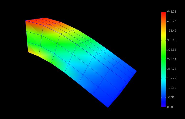
The following model extends FemBeam to render stress, with an added color bar. The loaded model is shown in Figure 1.23.
1.12.7 Cut planes
In addition to stress/strain visualization on its meshes, FEM models can be supplied with one or more cut planes that allow stress or strain values to be visualized on the cross section of the model with the plane.
Cut plane components are implemented by FemCutPlane and can be created with the following constructors:
| FemCutPlane() |
Creates a cut plane aligned with the world origin. |
| FemCutPlane (double res) |
Creates an origin-aligned cut plane with grid resolution res. |
| FemCutPlane (RigidTransform3d TPW) |
Creates a cut plane with pose TPW a specified grid resolution. |
| FemCutPlane (double res, RigidTransform3d TPW) |
Creates a cut plane with pose TPW and grid resolution res. |
The pose and resolution are described further below. Once created, a cut plane can be added to an FEM model using its addCutPlane() method:
The FEM model methods for handling cut planes include:
| void addCutPlane(FemCutPlane cp) |
Adds a cut plane to the model. |
| int numCutPlanes() |
Queries number of cut planes in the model. |
| FemCutPlane getCutPlanes(int idx) |
Gets the idx-th cut plane in the model. |
| boolean removeCutPlane(FemCutPlane cp) |
Removes a cut plane from the model. |
| void clearCutPlanes() |
Removes all cut planes from the model. |
As with rigid and mesh bodies, the pose of the cut plane gives
its position and orientation relative to world coordinates and is
described by a RigidTransform3d. The
plane itself is aligned with the ![]() -
-![]() plane of this local coordinate
system. More specifically, if the pose is given by
plane of this local coordinate
system. More specifically, if the pose is given by ![]() such that
such that
 |
(1.39) |
then the plane passes through point ![]() and its normal is given
by the
and its normal is given
by the ![]() axis (third column) of
axis (third column) of ![]() . When rendered in the
viewer, FEM model stress/strain values are displayed as a color map
within the polygonal region formed by the intersection between the
plane and the model’s surface mesh.
. When rendered in the
viewer, FEM model stress/strain values are displayed as a color map
within the polygonal region formed by the intersection between the
plane and the model’s surface mesh.
The following properties of FemCutPlane are used to control how it is rendered in the viewer:
- squareSize
-
A double value, which if
specifies the size of a square that
shows the position of the plane. - resolution
-
A double value, which if
specifies an explicit size (in units
of distance) for the grid cells created within the FEM surface/plane
intersection to interpolate stress/strain values. Smaller values will
give more accurate results but may slow down the rendering
time. Accuracy will also not be improved if the resolution is
significantly less that the size of the FEM elements. If resolution  , the grid size is determined automatically based
on the element sizes.
, the grid size is determined automatically based
on the element sizes. - axisLength, axisDrawStyle
-
Identical in function to the axisLength and axisDrawStyle properties for rigid bodies (Section LABEL:rigidBodyRendering:sec). Specifies the length and style for rendering the local coordinate frame of the cut plane.
- surfaceRendering
-
Describes what is rendered on the surface/plane intersection polygon, according to table 1.5.
- stressPlotRange, stressPlotRanging, colorMap
-
Identical in function to the stressPlotRange, stressPlotRanging and colorMap properties exported by FemModel3d and FemMeshComp (Section 1.12.3). Controls the range and color map associated with the surface rendering.
As with all properties, the values of the above can be accessed either in code using set/get accessors named after the property (e.g., setSurfaceRendering(), getSurfaceRendering()), or within the GUI by selecting the cut plane and then choosing Edit properties ... from the context menu.
1.12.8 Example: FEM model with a cut plane
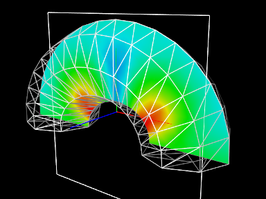
Cut planes are illustrated by the application model defined in
artisynth.demos.tutorial.FemCutPlaneDemo
which creates a simple FEM model in the shape of a half-torus, and then adds a cut plane to render its internal stresses. Its build() method is give below:
After a MechModel is created (lines 27-29), an FEM model
consisting of a half-torus is created, with the bottom nodes set
non-dynamic to provide support (lines 31-43). A cut plane is then
created with a pose that centers it on the world origin and aligns it
with the world ![]() -
-![]() plane (lines 47-49). Surface rendering is set
to Stress, with a fixed color plot range of
plane (lines 47-49). Surface rendering is set
to Stress, with a fixed color plot range of ![]() (lines
52-54). A control panel is created to expose various properties of the
plane (lines 57-63), and then other rendering properties are set: the
default FEM line color is made white (line 67); to avoid visual
clutter FEM elements are made invisible and instead the FEM is
rendered using a wireframe representation of its surface mesh (lines
69-74); and in addition to its render surface, the cut plane is also
displayed using its coordinate axes (with length 0.08) and a square of
size 0.12 (lines 76-78).
(lines
52-54). A control panel is created to expose various properties of the
plane (lines 57-63), and then other rendering properties are set: the
default FEM line color is made white (line 67); to avoid visual
clutter FEM elements are made invisible and instead the FEM is
rendered using a wireframe representation of its surface mesh (lines
69-74); and in addition to its render surface, the cut plane is also
displayed using its coordinate axes (with length 0.08) and a square of
size 0.12 (lines 76-78).
To run this example in ArtiSynth, select All demos > tutorial > FemCutPlaneDemo from the Models menu. When loaded and run, the model should appear as in Figure 1.24. The plane can be repositioned by selecting it in the viewer (by clicking on its square, coordinate axes, or render surface) and then using one of the transformer tools to change its position and/or orientation (see the section “Transformer Tools” in the ArtiSynth User Interface Guide).
![[LOGO]](data:image/png;base64,iVBORw0KGgoAAAANSUhEUgAAAAsAAAAOCAYAAAD5YeaVAAAAAXNSR0IArs4c6QAAAAZiS0dEAP8A/wD/oL2nkwAAAAlwSFlzAAALEwAACxMBAJqcGAAAAAd0SU1FB9wKExQZLWTEaOUAAAAddEVYdENvbW1lbnQAQ3JlYXRlZCB3aXRoIFRoZSBHSU1Q72QlbgAAAdpJREFUKM9tkL+L2nAARz9fPZNCKFapUn8kyI0e4iRHSR1Kb8ng0lJw6FYHFwv2LwhOpcWxTjeUunYqOmqd6hEoRDhtDWdA8ApRYsSUCDHNt5ul13vz4w0vWCgUnnEc975arX6ORqN3VqtVZbfbTQC4uEHANM3jSqXymFI6yWazP2KxWAXAL9zCUa1Wy2tXVxheKA9YNoR8Pt+aTqe4FVVVvz05O6MBhqUIBGk8Hn8HAOVy+T+XLJfLS4ZhTiRJgqIoVBRFIoric47jPnmeB1mW/9rr9ZpSSn3Lsmir1fJZlqWlUonKsvwWwD8ymc/nXwVBeLjf7xEKhdBut9Hr9WgmkyGEkJwsy5eHG5vN5g0AKIoCAEgkEkin0wQAfN9/cXPdheu6P33fBwB4ngcAcByHJpPJl+fn54mD3Gg0NrquXxeLRQAAwzAYj8cwTZPwPH9/sVg8PXweDAauqqr2cDjEer1GJBLBZDJBs9mE4zjwfZ85lAGg2+06hmGgXq+j3+/DsixYlgVN03a9Xu8jgCNCyIegIAgx13Vfd7vdu+FweG8YRkjXdWy329+dTgeSJD3ieZ7RNO0VAXAPwDEAO5VKndi2fWrb9jWl9Esul6PZbDY9Go1OZ7PZ9z/lyuD3OozU2wAAAABJRU5ErkJggg==)