Inverse Simulation

July 17, 2024

1 Inverse Simulation

Chapter 1 Inverse Simulation

1.1 Overview

ArtiSynth supports an inverse simulation capability that allows the computation of the excitation signals (for muscles and other actuators) needed to track target trajectories for a set of source components within the model (typically points or frames). This is achieved using a specialized controller component known as a TrackingController. An application model creates the tracking controller and configures it with the source components, the exciter components needed to effect the tracking, and probes or controllers to specify the target trajectories. Then at each simulation time step the controller computes the excitations (i.e., signals to the exciter components) that allow the trajectories to be followed as closely as possible, in a manner conceptually similar to computed muscle control in OpenSim [delp2007opensim].

1.1.1 Tracking controller operation

Let ${\bf q}$ , ${\bf u}$ and ${\bf f}$ be composite vectors describing the positions, velocities and forces of all the components in the application model, and let ${\bf a}$ be a vector of excitation signals for all the excitation components available to the controller. ${\bf f}$ can be decomposed into

${\bf f}={\bf f}_{p}({\bf q},{\bf u})+{\bf f}_{a}({\bf q},{\bf u},{\bf a})$

(1.1)

where ${\bf f}_{p}$ are the passive forces corresponding to zero excitation, and ${\bf f}_{a}$ are the active forces. During simulation, the controller computes values for ${\bf a}$ to best track the target trajectories.

In the case of motion tracking, let ${\bf x}$ and ${\bf v}$ be the subvectors of ${\bf q}$ and ${\bf u}$ containing the positions and velocities of the source components, and let ${\bf x}_{t}$ and ${\bf v}_{t}$ be the corresponding target trajectories. At the beginning of each time step, the controller compares the current source velocity state $({\bf x},{\bf v})$ with the desired target state $({\bf x}_{t},{\bf v}_{t})$ and uses this to determine a desired source velocity ${\bf v}_{*}$ for the next time step; this computation is done by the motion tracker (Figure 1.1, Section 1.1.2). An excitation generator then computes ${\bf a}$ in order to try and make ${\bf v}$ match ${\bf v}_{*}$ (Section 1.1.3).

The excitation generator accepts a desired velocity ${\bf v}_{*}$ instead of a desired acceleration because ArtiSynth’s physics engine computes velocity changes directly.

Figure 1.1: Tracking controller operation for motion targets.

1.1.2 Motion tracking

As mentioned above, the motion tracker computes a desired source velocity ${\bf v}_{*}$ for the next time step based on the current source state $({\bf x},{\bf v})$ and desired target state $({\bf x}_{t},{\bf v}_{t})$ . This can be done in two ways: chase control (the default), and PD control.

1.1.2.1 Chase control

Chase control simply sets ${\bf v}_{*}$ to ${\bf v}_{t}$ , plus an additional velocity that tries to reduce the position error ${\bf x}_{t}-{\bf x}$ over a specified time interval , called the chase time:

${\bf v}_{*}={\bf v}_{t}+\frac{{\bf x}_{t}-{\bf x}}{T}.$

(1.2)

In general, should be greater than or equal to the simulation step size . If it is greater, then ${\bf x}$ will tend to lag behind ${\bf x}_{t}$ , but this will also reduce the potential for overshoot due to system nonlinearities. Conversely, if if less than , then ${\bf x}$ is much more likely to overshoot. The default value of is 0.01.

1.1.2.2 PD control

PD control computes a desired source acceleration $\dot{\bf v}_{*}$ based on

$\dot{\bf v}_{*}=K_{p}({\bf x}_{t}-{\bf x})+K_{d}({\bf v}_{t}-{\bf v}),$

(1.3)

and then integrates this to determine ${\bf v}_{*}$ :

${\bf v}_{*}={\bf v}+h\dot{\bf v}_{*},$

(1.4)

where is the simulation step size. PD control offers a greater ability to adjust the tracking behavior than chase control, but it is often necessary to tune the gain parameters $K_{p}$ and $K_{d}$ . One rule of thumb is to set their initial values such that (1.2) and (1.4) are equal, which leads to

$K_{p}=\frac{1}{hT},\quad K_{d}=\frac{1}{h}.$

The default values for $K_{p}$ and $K_{d}$ are and , corresponding to and both equaling . Lowering the value of $K_{p}$ will reduce overshoot but increase tracking lag.

PD control is enabled and adjusted by setting the usePDControl, Kp and Kd properties of the motion target term to true (Section 1.3.3).

1.1.3 Generating excitations using a quadratic program

Given ${\bf v}_{*}$ , the excitation generator computes ${\bf a}$ to try and ensure that the velocity at the end of the subsequent time step, ${\bf v}^{k+1}$ , satisfies

${\bf v}^{k+1}\approx{\bf v}_{*}.$

(1.5)

This is accomplished using a quadratic program.

First, for a broad class of problems, ${\bf f}$ is linearly related to ${\bf a}$ , so that (1.1) simplifies to

${\bf f}={\bf f}_{p}({\bf q},{\bf u})+\Lambda({\bf q},{\bf u}){\bf a},$

(1.6)

where $\Lambda$ is an excitation response matrix. Given (1.6), it is possible to show (section “Inverse modeling” in [lloyd2012artisynth]) that

${\bf v}^{k+1}={\bf v}_{0}+{\bf H}_{m}{\bf a},$

where ${\bf v}_{0}$ is the velocity with zero excitations and ${\bf H}_{m}$ is a motion excitation response matrix. To best follow the trajectory, we can compute ${\bf a}$ to minimize the quadratic cost function

$\phi_{m}({\bf a})\equiv\frac{1}{2}\|{\bf v}_{*}-{\bf v}^{k+1}\|=\frac{1}{2}\|% \bar{\bf v}-{\bf H}_{m}{\bf a}\|^{2},\quad\bar{\bf v}\equiv{\bf v}_{*}-{\bf v}% _{0}.$

(1.7)

If we add in the constraint that excitations lie in the range , the problem takes the form of a quadratic program (QP)

	$\displaystyle\min_{{\bf a}}\;\phi_{m}({\bf a})$
	$\displaystyle\text{subject to}\quad 0\leq{\bf a}\leq{\bf 1}.$		(1.8)

In order to prioritize some target terms over others, $\phi_{m}({\bf a})$ can be modified to include weights, according to

$\phi_{m}({\bf a})\equiv\frac{1}{2}\|{\bf W}_{m}(\bar{\bf v}-{\bf H}_{m}{\bf a}% )\|^{2},$

(1.9)

where ${\bf W}_{m}$ is a diagonal weighting matrix. To handle excitation redundancy, where the size of ${\bf a}$ exceeds the size of ${\bf v}$ , we can add a regularization term $\frac{1}{2}{\bf a}^{T}{\bf W}_{a}{\bf a}$ , where ${\bf W}_{a}$ is a diagonal weight matrix that can be used to adjust the relative importance of specific excitations:

	$\displaystyle\min_{{\bf a}}\;\phi_{m}({\bf a})+\frac{1}{2}{\bf a}^{T}{\bf W}_{% a}{\bf a}$
	$\displaystyle\text{subject to}\quad 0\leq{\bf a}\leq{\bf 1}.$		(1.10)

The matrix ${\bf W}_{a}$ described here is the inverse of the matrix ${\bf W}$ presented in [lloyd2012artisynth].

1.1.4 Force tracking

Other cost terms can be added to the tracking controller. For instance, we can request a force trajectory ${\bf f}_{et}$ for a selected set of force effectors. As with motions, the forces of these effectors ${\bf f}_{e}$ at the end of step are linearly related to ${\bf a}$ via

${\bf f}_{e}^{k+1}={\bf f}_{e0}+{\bf H}_{e}{\bf a}$

where ${\bf f}_{t0}$ is the force with zero excitations and ${\bf H}_{e}$ is the force excitation response matrix. The force trajectory can then be tracking by minimizing

$\phi_{e}({\bf a})\equiv\frac{1}{2}\|{\bf W}_{e}(\bar{\bf f}_{e}-{\bf H}_{e}{% \bf a})\|^{2},\quad\bar{\bf f}_{e}\equiv{\bf f}_{et}-{\bf f}_{e0},$

(1.11)

where ${\bf W}_{e}$ is a diagonal weighting matrix. When tracking force targets, the target force trajectory ${\bf f}_{et}$ is fed directly into the excitation generator (Figure 1.2); there is no equivalent of the motion tracker.

Figure 1.2: Tracking controller operation for force targets.

To balance the effect of different cost terms, each is associated with a weight (e.g., $w_{m}$ , $w_{e}$ , and $w_{a}$ for the motion, force and regularization terms), so that the QP takes a form such as

	$\displaystyle\min_{{\bf a}}\;w_{m}\phi_{m}({\bf a})+w_{e}\phi_{f}({\bf a})+% \frac{w_{a}}{2}{\bf a}^{T}{\bf W}_{a}{\bf a}$
	$\displaystyle\text{subject to}\quad 0\leq{\bf a}\leq{\bf 1}.$		(1.12)

1.1.5 Incremental computation

In some cases, the system forces are not linear with respect to the excitations (i.e., equation (1.6) is not valid). One situitaton where this occurs is when equilbrium muscle models are used (Section LABEL:equilibriumMuscles:sec).

When forces are not linear in ${\bf a}$ , the force relationship can be linearized and the quadratic program can be reformulated in terms of excitation changes $\Delta{\bf a}$ ; for example,

	$\displaystyle\min_{\Delta{\bf a}}\;w_{m}\phi_{m}(\Delta{\bf a})+w_{e}\phi_{f}(% \Delta{\bf a})+\frac{w_{a}}{2}\Delta{\bf a}^{T}{\bf W}_{a}\Delta{\bf a}+{\bf a% }_{0}^{T}{\bf W}_{a}\Delta{\bf a}$
	$\displaystyle\text{subject to}\quad-{\bf a}_{0}\leq\Delta{\bf a}\leq{\bf 1-{% \bf a}_{0}}.$		(1.13)

where ${\bf a}_{0}$ denotes the excitation values at the beginning of the time step. Excitations are then updated according to

${\bf a}={\bf a}_{0}+\Delta{\bf a}.$

Incremental computation can be enabled, at the expense of slower computation, by setting the tracking controller property computeIncrementally to true (Section 1.3.2).

1.1.6 Setting up the tracking controller

Applications will generally set up a tracking controller using the following steps inside the application’s build() method:

1.

Create an instance of TrackingController and add it to the application using the root model’s addController() method.
2.

Configure the controller with the available excitation components using its addExciter(ex) and addExciter(weight,ex) methods.
3.

Configure the controller to track position or force trajectories for selected source components, which may include Point, Frame, or ForceEffector components. These are specified to the controller using methods such as addPointTarget(point), addFrameTarget(frame), and addForceEffectorTarget(forceEffector). These methods return a target object, which is allocated and maintained by the controller, and which is used for specifying the target positions or forces.
4.

Create input probes or controllers to specify the desired trajectories for the sources added in Step 3. Trajectories are specified by using probes or controllers to set the appropriate target properties of the target objects returned by the addXXXTarget() methods. Likewise, output probes or monitors can be created to record the excitations and the tracked positions or forces of the sources.
5.

Add other cost terms as needed. These may include an L2 regularization term, added using the controller’s addL2RegularizationTerm() method. Regularization attempts to minimze the norm of the excitation values and is needed to resolve redundancy if the excitation set has more degrees of freedom that the target space.
6.

Set controller configuration parameters.

Once the tracking controller has been set up, during subsequent simulation it will compute excitation values, using the quadratic program described in Sections 1.1.3 and 1.1.4, so as to best follow the prescribed target trajectories.

1.1.7 Example: moving a point with multiple Muscles

Figure 1.3: InverseParticle when first loaded (left), and during simulation with the muscles activated to move the center particle (right).

Figure 1.4: Probes showing the target position and computed excitations for InverseParticle.

An simple example illustrating the steps of Section 1.1.6 is given by

  artisynth.demos.tutorial.InverseParticle

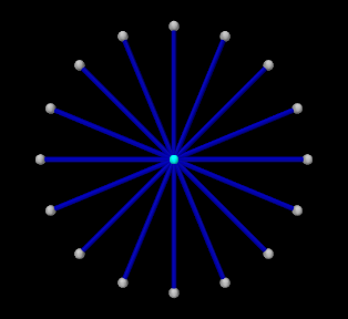
which uses a set of point-to-point muscles to drive the position of a single particle. The model consists of a single dynamic particle, initially located at the origin, attached to a set of 16 point-to-point muscles arranged radially around it. A tracking controller is created to control the excitations of these muscles so as to enable the particle to follow a trajectory specified by a probe. The code for the model, without the package and include directives, is listed below:

⬇

1 public class InverseParticle extends RootModel {

3 int numMuscles = 16; // num radial muscles surrounding the dynamic particle

4 double muscleStiffness = 200; // passive muscle stiffness

5 double muscleDamping = 1.0; // passive muscle damping

6 double muscleFmax = 1000; // max active force at excitation = 1

7 double dist = 1.0; // distance of anchor point from world origin

9 /**

10 * Create a muscle excitable spring extending out from the origin

11 * {@code part} at an angle {@code ang}.

12 */

13 void createMuscle (MechModel mech, Particle part, double ang) {

14 // create and add non-dynamic particle as fixed end point for muscle

15 Particle fixed = new Particle(

16 /*mass=*/1d, new Point3d(dist*Math.sin(ang),0.0,dist*Math.cos(ang)));

17 fixed.setDynamic(false);

18 mech.addParticle(fixed);

19 // create muscle and set its material

20 Muscle muscle = new Muscle (fixed, part);

21 muscle.setName ( // name the muscle using its angle

22 "muscle_"+Integer.toString((int)Math.round(Math.toDegrees(ang))));

23 muscle.setMaterial (

24 new SimpleAxialMuscle (muscleStiffness, muscleDamping, muscleFmax));

25 mech.addAxialSpring (muscle);

27 // make muscles red when activated

28 muscle.setExcitationColor (Color.RED);

29 muscle.setMaxColoredExcitation (0.5);

30 muscle.setRestLength (muscle.getLength());

31 }

33 public void build (String[] args) {

34 // create MechModel and add to RootModel

35 MechModel mech = new MechModel ("mech");

36 addModel (mech);

37 mech.setGravity (Vector3d.ZERO); // disable gravity

39 // create and add particle whose position is to be controlled

40 Particle part = new Particle ("center", /*mass=*/0.1, /*x,y,z=*/0, 0, 0);

41 part.setPointDamping (0.1); // add damping

42 mech.addParticle(part);

44 // create radial muscles connected to center particle

45 for (int i = 0; i < numMuscles; i++) {

46 double angle = 2*Math.PI*((double)i/numMuscles);

47 createMuscle (mech, part, angle);

48 }

50 // create the tracking controller and add it to the root model

51 TrackingController tcon = new TrackingController(mech, "tcon");

52 addController(tcon);

53 // set all muscles to be "exciters" for the controller to control

54 for (AxialSpring s : mech.axialSprings()) {

55 if (s instanceof Muscle) {

56 tcon.addExciter((Muscle)s);

57 }

58 }

59 // set the center dynamic particle to be the component that is tracked

60 TargetPoint target = tcon.addPointTarget(part);

61 // add an L-2 regularization term, since there are more muscles than

62 // target degrees-of-freedom

63 tcon.addL2RegularizationTerm(/*weight=*/0.1);

65 // Render properties: make points gray spheres, central particle white,

66 // and muscles as blue cylinders.

67 RenderProps.setSphericalPoints (this, dist/25, Color.LIGHT_GRAY);

68 RenderProps.setPointColor (part, Color.WHITE);

69 RenderProps.setCylindricalLines (mech, dist/50, Color.BLUE.darker ());

71 // add an input probe to control the position of the target:

72 NumericInputProbe targetprobe = new NumericInputProbe (

73 target, "position", /*startTime=*/0, /*stopTime=*/1);

74 targetprobe.setName ("target positions");

75 targetprobe.addData (

76 new double[] {0d,0d,0d, 0.5,0d,0.5, 0d,0d,0d}, // three knot points

77 /*timestep=*/0.5);

78 targetprobe.setInterpolationOrder (Interpolation.Order.Cubic);

79 addInputProbe (targetprobe);

81 // add an output probe to record the excitations:

82 NumericOutputProbe exprobe = InverseManager.createOutputProbe (

83 tcon, ProbeID.COMPUTED_EXCITATIONS, /*fileName=*/null,

84 /*startTime=*/0, /*stopTime=*/1, /*interval=*/-1);

85 addOutputProbe (exprobe);

86 }

87 }

The build() method begins by creating a MechModel in the usual way and disabling gravity (lines 35-37). The particle to be controlled is then created and placed at the origin and with a damping factor of 0.1 (lines 40-42). Next, the particle is attached to a set of point-to-point muscles that are arranged radially around it (lines 45-48). These are created using the method createMuscle() (lines 13-31), which attaches each to a fixed non-dynamic particle located a distance of dist from the origin, and sets its material to a SimpleAxialMuscle (Section LABEL:SimpleAxialMuscle:sec) with a passive stiffness, damping and maximum force (at excitation 1) defined by muscleStiffness, muscleDamping, and muscleFmax (lines 4-6). Each muscle’s excitationColor and maxColoredExcitation property is set so that its color transitions to red as its excitation value varies from to (lines 28-29, Section 1.2.1.1)), and its rest length is initialized to its current length (line 30).

After the model components have been built, a TrackingController is created and added to the root model’s controller set (lines 51-52). All of the muscles are then added to the controller as exciters to be controlled (lines 54-58). The particle is added to the controller as a motion source using the addPointTarget() method (line 60), which returns a target object in the form of a TargetPoint. Since the number of exciters exceeds the degrees-of-freedom of the target space, an L2-regularization term is added (line 63) to resolve the redundancy.

Rendering properties are set at lines 67-69: points in the model are rendered as gray spheres, except for the dynamic particle which is colored white, and the muscles are drawn as blue cylinders. (The target particle, which is contained within the controller, is displayed using its default color of cyan.)

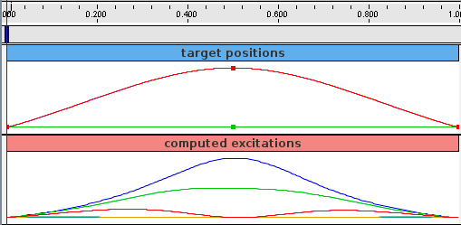
Probes are created to specify the target trajectory and record the computed excitations. The first, targetprobe, is an input probe attached to the position property of the target component, running from time 0 to 1 (lines 72-79). Its data is specified in code using addData(), which specifies three knot points with a time step of 0.5. Interpolation is set to cubic (line 78) for greater smoothness. The second, exprobe, is a probe that records all the excitations computed by the controller (lines 82-85). It is created by the utility method createOutputProbe() supplied by the InverseManager class (Section 1.4.1).

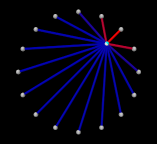
To run this example, select All demos > tutorial > InverseParticle from the Models menu. The model should load and initially appear as in Figure 1.3 (left). When run, the controller computes excitations to move the particle along the trajectory specified by the probe, which is upward and to the right (Figure 1.3, right) and back again.

The target point created by the controller is rendered separately from the source point as a cyan-colored sphere (see Section 1.2.2.2). As the simulation proceeds and certain muscles are excited, their coloring changes from blue to red, in proportion to their excitation, in accordance with the properties excitationColor and maxColoredExcitation. Recorded data for both the trajectory and the computed excitation probes are shown in Figure 1.4.

1.2 Tracking controller components

This section describes in greater detail how exciters, motion and force sources, and other cost terms can be specified for the controller.

1.2.1 Exciters

An exciter can be any model component that implements ExcitationComponent. These include point-to-point Muscles (Section LABEL:PointToPointMuscles:sec), muscle bundles in FEM muscle models (Section LABEL:MuscleBundles:sec), and MuscleExciters (Section LABEL:MuscleExciters:sec). Each exciter exports an excitation property which accepts a scaler input signal (usually in the range ) that drives the exciter’s active force (or fans it out to other exciters in the case of a MuscleExciter).

The set of excitation components used by a tracking controller is managed by the following methods:

void addExciter(ExcitationComponent ex)	Adds an exciter with default weight 1.0.
void addExciter(double w, ExcitationComponent ex)	Adds an exciter with weight w.
void addExciters(Collection<ExcitationComponent> exciter)	Adds a collection of exciters with weights 1.0.
int numExciters()	Returns the number of exciters.
ExcitationComponent getExciter (int idx)	Returns the idx-th exciter.
ArrayList<ExcitationComponent> getExciters()	Returns a list of all exciters.
void clearExciters()	Remove all exciters.

An exciter’s weight forms its corresponding entry in the diagonal matrix ${\bf W}_{a}$ used by the quadratic program ((1.10 and (1.12)), with a smaller weight allowing the exciter to assume greater prominence in the solution.

By default, the computed excitations are bounded by the interval , as indicated in Section 1.1.3. However, these bounds can be altered, either collectively using the tracking controller property excitationBounds, or individually for specific exciters:

void setExcitationBounds(DoubleInterval range)	Sets the excitationBounds property.
DoubleInterval getExcitationBounds()	Queries the excitationBounds property.

void setExcitationBounds(ExcitationComponent ex, Mdouble low, double high)	Sets excitation bounds for exciter ex.
DoubleInterval getExcitationBounds(ExcitationComponent ex)	Queries excitation bounds for exciter ex.

The excitation values themselves can also be queried and set with the following methods:

void getExcitations(VectorNd values)	Returns excitations in values.
double getExcitation(int idx)	Returns the excitation of the idx-th exciter.

By default, the controller initializes excitations to zero and then updates them at the beginning of each time step. However, when excitations are being computed incrementally (Section 1.1.5), it may be desirable to start with non-zero excitation values. In that case, the following methods may be useful:

void initializeExcitations()	Sets excitations to the current exciter values.
void setExcitations(VectorNd values)	Sets excitations to values.

The first sets the controller’s internal excitation values to those stored in the exciters, while the second sets both the internal values and the values in the exciters.

1.2.1.1 Excitation coloring

Some exciters (such as Muscle and MultiPointMuscle) support the ability to change color in proportion to their excitation value. This makes it easier to visualze the extent to which exciters are being activated within the model. Exciters which support this capability export the properties excitationColor, which is the color the exciter should transition to as excitation is increased, and maxColoredExcitation, which the excitation value at which the color transition is complete. In other words, the exciter’s color will vary from its default color to excitationColor as its excitation varies from 0 to maxColoredExcitation.

Excitation coloring does not occur if the exciter’s excitationColor is set to null.

The tracking controller exports a property, configExcitationColoring, which if true enables the automatic configuration of excitation coloring for exciters that support this capability. If enabled, then as these exciters are added to the controller, their excitationColor is inspected. If it has not been set (i.e., if it is null), then it is set to red and the nominal color for the exciter is set to white, enabling a white-to-red color transition for the exciter as it is activated.

1.2.2 Motion targets

As indicated above, motion source components can be specified to the controller using the addPointTarget() and addFrameTarget() methods. Source components may be instances of Point or Frame, and thereby may include both FEM nodes and rigid bodies. The methods for managing motion targets include:

TargetPoint addPointTarget(Point source)	Adds point source with weight 1.0.
TargetPoint addPointTarget(Point source, double w)	Adds point source with weight w.
TargetFrame addFrameTarget(Frame source)	Adds frame source with weight 1.0.
TargetFrame addFrameTarget(Frame source, double w)	Adds frame source with weight w.

int numMotionTargets()	Number of motion targets.
void removeMotionTarget(MotionTargetComponent source)	Removes motion source.

The addPointTarget() and addFrameTarget() methods each create and return a target component, allocated and contained within the controller, that mirrors the type of source component. These target components are either TargetPoint for point sources or TargetFrame for frame sources. Both TargetPoint and TargetFrame, together with the source components Point and Frame, are instances of MotionTargetComponent.

As simulation proceeds, the desired trajectory position ${\bf x}_{t}$ for each source component is specified by setting the target component’s position property (or position, orientation and/or pose properties for frame targets). As described elsewhere, this can be done using either probes or other controller objects.

Likewise, a corresponding velocity trajectory ${\bf v}_{t}$ can also be specified by setting the velocity property of the target object. If this is not set, ${\bf v}_{t}$ defaults to 0, which will introduce a small lag into the tracking behavior. If ${\bf v}_{t}$ is set, care should be taken the ensure that it is consistent with the actual time derivative of ${\bf x}_{t}$ .

Applications typically do not need to specify ${\bf v}_{t}$ . However, doing so may improve tracking performance, particularly when using PD control (Section 1.1.2).

Each target component also implements the interface TrackingTarget, described in Section 1.2.8, which supplies methods to specify the weights in the weighting matrix ${\bf W}_{m}$ of the motion tracking cost term $\phi_{m}({\bf a})$ (1.9).

Lists of all the motion source components and their associated target components (i.e., those returned by the addXXXTarget() methods) can be obtained using

ArrayList<MotionTargetComponent> getMotionSources()	Returns motion source components.
ArrayList<MotionTargetComponent> getMotionTargets()	Returns motion target components.

1.2.2.1 Motion target term

The cost term $\phi_{m}({\bf a})$ that is responsible for tracking motion targets is contained within a tracking controller subcomponent that is named "motionTerm" and which is an instance of MotionTargetTerm. Users may access this component directly using

MotionTargetTerm getMotionTargetTerm()

Returns the controller’s motion target term.

and then use it to set motion tracking properties such as those described in Section 1.3.3.

The motion tracking weight $w_{m}$ in (1.12) is given by the weight property of the motion target term, which can also be accessed directly by the controller methods

double getMotionTargetTermWeight()	Returns the motion target term weight.
void setMotionTargetTermWeight(double w)	Sets the motion target term weight.

1.2.2.2 Motion target rendering

The motion target components, which are allocated and maintained by the controller, are rendered by default, which makes it easy to visualize significant errors between the target positions and the trackes source positions. Target points are drawn as cyan colored spheres. For target frames, if the source component corresponds to a RigidBody, the target is rendered using a cyan colored wireframe copy of the source’s surface mesh.

Rendering of targets can be enabled or disabled by setting the tracking controller’s targetsVisible property. Otherwise, the application is free to set the render properties of individual target components, or their containing lists within the MotionTargetTerm, which can be accessed by the methods

PointList<TargetPoint> getTargetPoints()	Return all point motion target components.
RenderableComponentList<TargetFrame> getTargetFrames()	Return all frame motion target components.

Other methods of MotionTargetTerm allow the render properties for both the point and frame target lists to be set together:

RenderProps getTargetRenderProps()	Return render properites for the motion target lists.
void setTargetRenderProps (RenderProps props)	Set render properites for the motion target lists.
void setTargetsPointRadius (double rad)	Set pointRadius target render property to rad.

1.2.3 Regularization

1.2.3.1 L2 Regularization

L2 regularization attempts to minimize the weighted square of the excitation values, as described by

$\frac{w_{a}}{2}\,{\bf a}^{T}{\bf W}_{a}\,{\bf a}$

(1.14)

in (1.12), and so provides a way to resolve redundancy when the number of exciters is greater than needed to perform the required tracking. It can be enabled or disabled by adding or removing an L2 regularization term from the controller, as managed by the following methods:

void addL2RegularizationTerm()	Add L2 regularization with weight 1.0.
void addL2RegularizationTerm(double w)	Add L2 regularization with weight w.
void removeL2RegularizationTerm()	Remove L2 regularization.

The weight associated with the above methods corresponds to $w_{a}$ in (1.14) and (1.12). The entries in the diagonal matrix ${\bf W}_{a}$ are given by the weights associated with the exciters themselves, as described in Section 1.2.1.

L2 regularization is implemented using a controller subcomponent of type L2RegularizationTerm, which is added or removed from the controller as required and can be accessed using

L2RegularizationTerm getL2RegularizationTerm()

Returns the controller’s L2 regularization term

which will return null if regularization is not being applied.

Because the L2 regularizer tries to reduce the excitations ${\bf a}$ , its use will reduce the controller’s tracking accuracy. Therefore, the regularizer is often employed with a weight value $w_{a}$ well below 1.0, with values around 0.1 or 0.01 being common. The best weight choice will of coarse depend on the application.

1.2.3.2 Excitation damping

The controller also provides a damping term that serves to minimize the time derivative of ${\bf a}$ , or more precisely,

$\frac{1}{2}\dot{\bf a}^{T}{\bf W}_{a}\dot{\bf a},$

where ${\bf W}_{a}$ is the diagonal excitation weight matrix used for L2 regularization (1.14). Letting ${\bf a}_{0}$ denote the excitations at the beginning of the time step, and approximating $\dot{\bf a}$ by

$\dot{\bf a}\approx\frac{{\bf a}-{\bf a}_{0}}{h},$

where is the time step size, the damping cost term $\phi_{d}({\bf a})$ becomes

$\phi_{d}({\bf a})=\frac{1}{2h^{2}}\left({\bf a}^{T}{\bf W}_{a}{\bf a}-2{\bf a}% _{0}^{T}{\bf W}_{a}{\bf a}\right).$

Excitation damping can be managed by the following methods:

void addDampingTerm()	Add excitation damping with weight 1.0.
void addDampingTerm(double w)	Add excitation damping with weight w.
void removeDampingTerm()	Remove excitation damping.

Excitation damping is implemented using a controller subcomponent of type DampingTerm, which is added or removed from the controller as required and can be accessed using

DampingTerm getDampingTerm()

Returns the controller’s excitation damping.

which will return null if damping is not being applied.

1.2.4 Example: controlling ToyMuscleArm

Figure 1.5: InverseMuscleArm when first loaded into ArtiSynth.

A good tracking controller example is given by the model artisynth.demos.tutorial.InverseMuscleArm, which computes the muscle excitations needed to make the tip marker of the ToyMuscleArm demo (described in Section LABEL:ToyMuscleArm:sec) follow a presribed trajectory. The model extends artisynth.demos.tutorial.ToyMuscleArm, and then adds the tracking controller and probes needed to move the tip marker, as shown in the code below:

⬇

1 public class InverseMuscleArm extends ToyMuscleArm {

3 public void build (String[] args) throws IOException {

4 super.build(args); // create ToyMuscleArm

6 // move the model into a non-singular position so it can track a target

7 // trajectory more easily

8 myHinge0.setTheta (-20);

9 myHinge1.setTheta (38.4);

10 myMech.updateWrapSegments(); // update muscle wrapping for new config

12 // Create a tracking controller

13 TrackingController tcon = new TrackingController (myMech, "tcon");

14 addController (tcon);

15 // For each muscle, reinitialize its rest length for the new

16 // configuration and add it to the controller as an exciter

17 for (AxialSpring spr : myMech.axialSprings()) {

18 spr.setRestLength (spr.getLength());

19 tcon.addExciter ((Muscle)spr);

20 }

21 for (MultiPointSpring spr : myMech.multiPointSprings()) {

22 spr.setRestLength (spr.getLength());

23 tcon.addExciter ((MultiPointMuscle)spr);

24 }

26 // Add the tip marker to the controller as a motion target

27 TargetPoint target = tcon.addPointTarget (myTipMkr);

28 // add an L-2 regularization term to handle exciter redundancy

29 tcon.addL2RegularizationTerm(/*weight=*/0.1);

31 double startTime = 0; // probe start times

32 double stopTime = 5; // probe stop times

33 // Specify a target trajectory for the tip marker using an input probe.

34 NumericInputProbe targetprobe = new NumericInputProbe (

35 target, "position", startTime, stopTime);

36 targetprobe.setName ("target positions");

37 double x0 = 0; // initial x coordinate of the marker

38 double z0 = 1.1806; // initial z coordinate of the marker

39 double xmax = 0.6; // max x coordinate of the trajectory

40 // Trajectory data: five cubically interpolated knot points, running for

41 // 5 seconds, giving a closed loop shape:

42 targetprobe.addData (new double[] {

43 x0,0,z0, xmax,0,z0-0.2, x0,0,z0-0.4, -xmax,0,z0-0.2, x0,0,z0},

44 /*timestep=*/stopTime/4);

45 targetprobe.setInterpolationOrder (Interpolation.Order.Cubic);

46 addInputProbe (targetprobe);

48 // add an output probe to record the excitations:

49 NumericOutputProbe exprobe = InverseManager.createOutputProbe (

50 tcon, ProbeID.COMPUTED_EXCITATIONS, /*fileName=*/null,

51 startTime, stopTime, /*interval=*/-1);

52 addOutputProbe (exprobe);

54 // add tracing probes to view both the tracking target (in cyan) and the

55 // actual tracked position (in red).

56 TracingProbe tprobe;

57 tprobe = addTracingProbe (target, "position", startTime, stopTime);

58 tprobe.setName ("target tracing");

59 RenderProps.setLineColor (tprobe, Color.CYAN);

60 tprobe = addTracingProbe (myTipMkr, "position", startTime, stopTime);

61 tprobe.setName ("source tracing");

62 RenderProps.setLineColor (tprobe, Color.RED);

64 // add inverse control panel

65 InverseManager.addInversePanel (this, tcon);

66 // settings to allow probe management by InvereManager:

67 tcon.setProbeDuration (stopTime); // default probe duration

68 // set working folder for probe files

69 ArtisynthPath.setWorkingFolder (

70 new File (PathFinder.getSourceRelativePath (this, "inverseMuscleArm")));

71 }

72 }

As mentioned above, this model extends ToyMuscleArm (line 1), and so calls super.build(args) in the build() method to create all the components of ToyMuscleArm. Once this is done, the link positions are adjusted by setting the hinge joint angles (lines 8-9); this is done to move the arm away from the kinematic singularity at full extension and thus make it easier for the tip to follow a prescribed path. After the links are moved, the all wrap paths are updated by calling the MechModel method updateWrapPath() (line 10).

A tracking controller is then created (lines 13-14), and every Muscle and MultiPointMuscle is added to it as an exciter (lines 17-24). When iterating through the muscles, their rest lengths are reinitialized to their current lengths (which changed when the links were repositioned) to ensure that passive muscle forces are zero in the initial position.

Next, the marker at the tip of link1 (referenced by the inherited attribute myTipMarker) is added to the controller as a motion source (line 27) and the returned target object is stored in target. An L2 regularization term is added to the controller with weight 0.01 (line 29), and an input probe is created to provide the marker trajectory by setting the target’s position property (lines 31-46). The probe has a duration of 5 seconds, and the trajectory is a closed path, specified by 5 cubically interpolated knot points (line 43), that lie in the x-z plane and start at and return to the marker’s initial position x0, z0.

Probes are created to record the computed excitations and trace the desired and actual trajectories in the viewer. The first, exprobe, is created by the utility method createOutputProbe() supplied by the InverseManager class (lines 49-52, Section 1.4.1). The tracing probes are created by the RootModel method addTracingProbe() (lines 56-62), and two are created: one to trace the desired target by recording the position property of target, and another to trace the actual tracked (source) position by recording the position property of myTipMkr. The line colors of these are set to cyan and red, respectively, which specifies their display color in the viewer.

Lastly, an inverse control panel (Section 1.4.3) is created to manage controller properties (line 65), and some settings are made to allow for probe management by the InverseManager class, as discussed in Section 1.4.1 (lines 67-70); this includes setting the default probe duration to stopTime and the working folder to inverseMuscleArm located under the source folder.

Figure 1.6: InverseMuscleArm run with L2 regularization weights of 0.1 (left) and 10 (right). Traces of the desired and actual trajectories are shown in cyan and red, respectively, and computed excitation values are shown in graphs below. A regularization weight of 10results in a larger tracking error.

To run this example, select All demos > tutorial > InverseMuscleArm from the Models menu. The model should load and initially appear as in Figure 1.5. When run, the controller will compute excitations to make the tip marker trace the desired trajectory, as shown in Figure 1.6 (left), where the tracing probe shows the target trajectory in cyan; the source trajectory appears beneath it in red but is largely invisible because it follows the target quite accurately. Computed excitation values are shown below. The target component created for the tip marker is rendered as a cyan-colored sphere (Section 1.2.2.2).

The muscles in InverseMuscleArm are initially colored white instead of red (as they are for ToyMuscleArm). That is because if a muscle’s excitationColor property is null, the controller automatically configures the muscle to vary in color from white to red as the muscle is activated, as described in Section 1.2.1.1. This behaviour can be disabled by setting the controller property configExcitationColoring to false.

To illustrate how the L2 regularization weight can affect the tracking error, 1.6 (right) shows the model run with a regularization weight of 10 instead of 0.1. The tracking error is now visible, with the red source trace probe clearly distinct from the cyan target trace. The computed muscle excitations are also noticably different.

1.2.5 Example: controlling an FEM muscle model

Figure 1.7: InverseMuscleFem when first loaded into ArtiSynth (left), and after executing in the inverse simulation (right).

Another example involving an FEM muscle model is given by artisynth.demos.tutorial.InverseMuscleFem, which computes the muscle excitations needed to make an attached frame of the ToyMuscleFem demo (described in Section LABEL:ToyMuscleFem:sec) follow a presribed trajectory.

The model extends artisynth.demos.tutorial.ToyMuscleFem, and then adds the tracking controller and probes needed to move the tip marker, as shown in the code below:

⬇

1 public class InverseMuscleFem extends ToyMuscleFem {

3 protected String dataDir = PathFinder.getSourceRelativePath (this, "data/");

5 public void build (String[] args) throws IOException {

6 super.build (args); // build the underlying ToyMuscleFem model

8 // create a tracking controller

9 TrackingController tcon = new TrackingController (myMech, "tcon");

10 addController (tcon);

11 // add each FEM muscle bundle to it as an exciter

12 for (MuscleBundle b : myFem.getMuscleBundles()) {

13 tcon.addExciter (b);

14 }

15 // add the frame attached to the FEM as a motion target

16 TargetFrame target = tcon.addFrameTarget (myFrame);

18 // add an L-2 regularization term to handle exciter redundancy

19 tcon.addL2RegularizationTerm(/*weight=*/0.1);

20 // set the controller motion term to use PD control

21 tcon.getMotionTargetTerm().setUsePDControl (true);

22 tcon.getMotionTargetTerm().setKp (1000);

23 tcon.getMotionTargetTerm().setKd (100);

25 // add input probes specifying the desired position and orientation

26 // trajectory of the target:

27 double startTime = 0;

28 double stopTime = 5;

29 NumericInputProbe tprobePos =

30 new NumericInputProbe (

31 target, "position", dataDir+"inverseFemFramePos.txt");

32 tprobePos.setName ("target frame position");

33 addInputProbe (tprobePos);

34 NumericInputProbe tprobeRot =

35 new NumericInputProbe (

36 target, "orientation", dataDir+"inverseFemFrameRot.txt");

37 tprobeRot.setName ("target frame orientation");

38 addInputProbe (tprobeRot);

40 // add output probes showing the tracked position and orientation of the

41 // target frame source:

42 NumericOutputProbe sprobePos =

43 new NumericOutputProbe (

44 myFrame,"position", startTime, stopTime, /*interval*/-1);

45 sprobePos.setName ("source frame position");

46 addOutputProbe (sprobePos);

47 NumericOutputProbe sprobeRot =

48 new NumericOutputProbe (

49 myFrame,"orientation", startTime, stopTime, /*interval*/-1);

50 sprobeRot.setName ("source frame orientation");

51 addOutputProbe (sprobeRot);

53 // add an output probe to record the excitations:

54 NumericOutputProbe exprobe = InverseManager.createOutputProbe (

55 tcon, ProbeID.COMPUTED_EXCITATIONS, /*fileName=*/null,

56 startTime, stopTime, /*interval=*/-1);

57 addOutputProbe (exprobe);

58 // create a control panel for the controller

59 InverseManager.addInversePanel (this, tcon);

60 }

61 }

Since the model extends ToyMuscleFem (line 1), the build() method begins by calling super.build(args) to create the model defined by the superclass. A tracking controller is then created and added to the root model’s controller set, all the muscle bundles in the FEM muscle model are added to it as exciters, and the attached frame is added to it as a motion source using addFrameTarget (lines 9-16).

An L2 regularization term is added, and then the motion tracking is set to use PD control (Section 1.1.2), using gains of $K_{p}=1000$ and $K_{d}=100$ (line 19-23).

To control position and orientation of the frame, two input probes are created (lines 27-38), one attached to the target’s position and the other to its orientation. (While it is possible to use a single probe to control both of these properties, or the single pose property, separate probes are used here to provide easier visualization.) Their data and settings are read from the probe files inverseFemFramePos.txt and inverseFemFrameRot.txt, located in the folder data beneath the application model source folder. Each specifies a probe in tne time range from 0 to 5, with 26 knot points and cubic interpolation.

Figure 1.8: Probe data generated by InverseMuscleFem. Top: target trajectory for the frame position (26 knot points, cubiclly interpolated). Middle: actual position tracked by the controller. Bottom: computed muscle excitations.

To monitor the controller’s tracking performance, two output probes are created and attached to the position and orientation properties of the source component myFrame (lines 58-67). Setting the interval argument to -1 in the probes’ constructors causes them to use the model’s current step size as the update interval. Finally, the utility class InverseManager (Section 1.4) is used to create an output probe for the computed excitations, as well as a control panel giving access to the various controller properties (lines 70-75).

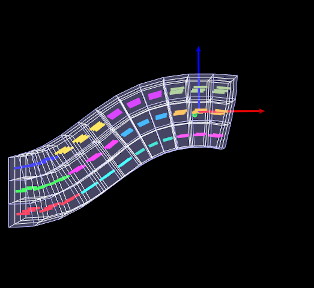
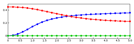
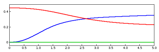
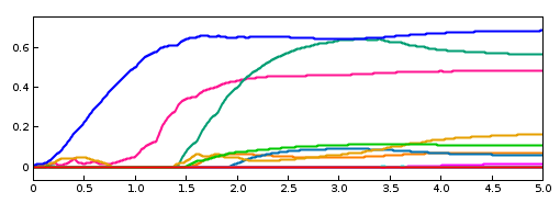
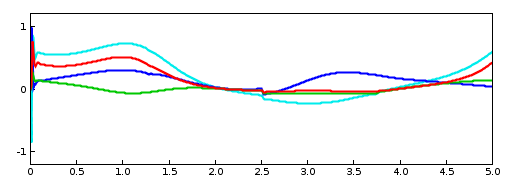
To run this example, select All demos > tutorial > InverseMuscleFem from the Models menu. The model should load and initially appear as in Figure 1.7 (left). When run, the controller will compute excitations to move the attached frame along the specified position/orientation trajectory, reaching the final pose shown in Figure 1.7 (right). The target and actual source trajectories for the frame’s position (i.e., its origin) is shown in Figure 1.8, together with the computed excitations.

1.2.6 Force effector targets

The controller can also be asked to track a force trajectory for a set of force effector components; the excitations will then be computed to try to generate the prescribed forces. Any force component that implements the interface ForceTargetComponent can be used as a force effector source; this interface extends ForceEffector to supply several additional methods including:

⬇

interface ForceTargetComponent extends ForceEffector, ModelComponent {

// gets the dimension of the generated force

public int getForceSize();

// returns the current force value

public void getForce (VectorNd minf, boolean staticOnly);

...

}

At the time of this writing, ForceTargetComponents include:

Component	Force size	Force description
AxialSpring	1	Tension in the spring
Muscle	1	Tension in the muscle
FrameSpring	6	Spring wrench as seen in body A (world coordinates)

Controller methods for adding and managing force effector targets include:

ForceEffectorTarget addForceEffectorTarget ( MForceTargetComponent source)	Adds static-only force source with weight 1.0
ForceEffectorTarget addForceEffectorTarget ( MForceTargetComponent source, double w)	Adds static-only force source with weight w.
ForceEffectorTarget addForceEffectorTarget ( MForceTargetComponent source, double w, boolean staticOnly)	Adds force source with weight w and static-only specified.

int numForceEffectorTargets()	Number of force effector targets.
boolean removeForceEffectorTarget( MForceTargetComponent source)	Removes force source.

The addForceEffectorTarget() methods each create and return a ForceEffectorTarget component. As simulation proceeds, the desired target force for the source component is specified by setting the target component’s targetForce property. As described elsewhere, this can be done using either probes or other controller objects. The target component also implements the interface TrackingTarget, described in Section 1.2.8, which supplies methods to specify the weighting matrix ${\bf W}_{e}$ in the force effector cost term $\phi_{e}({\bf a})$ (1.11).

By default, force effector tracking is static-only, meaning that only static forces (i.e., forces that are not velocity dependent, such as damping) are considered. However, the third addForceEffectorTarget() method allows this to be explictly specified.

Lists of all the force effector source components and their associated targets can be obtained using the methods:

ArrayList<ForceEffectorTarget> getForceEffectorSources()	Returns force effector source components.
ArrayList<ForceEffectorTarget> getForceEffectorTargets()	Returns force effector target components.

Specifying a force effector targetForce of 0 will have the same effect as minimizing the force associated with that force effector.

1.2.6.1 Force effector term

The cost term $\phi_{e}({\bf a})$ that is responsible for tracking force effector targets is contained within a tracking controller subcomponent named "forceEffectorTerm" and which is an instance of ForceEffectorTerm. This is added to the controller automaticlly whenever force effector tracking is requested, and may accessed directly using

ForceEffectorTerm getForceEffectorTerm()

Returns the force effector term.

The method will return null if the force effector term is not present.

The force effectior tracking weight $w_{e}$ in (1.12) is given by the weight property of the force effector term, which can also be accessed directly by the controller methods

double getForceEffectorTermWeight()	Returns the force effector term weight.
void setForceEffectorTermWeight(double w)	Sets the force effector term weight.

1.2.7 Example: controlling tension in a spring

Figure 1.9: InverseSpringForce when first loaded (left), and during simulation with the lower muscles fully activated to control the tension in the upper passive spring (cyan).

A simple example of force effector tracking is given by

  artisynth.demos.tutorial.InverseSpringForce

which uses two point-to-point muscles to control the tension in a passive spring. The initial part of the code is the same as that for InverseParticle (Section 1.1.7), except for different parameter defintions,

⬇

int numMuscles = 3; // num radial muscles surrounding the dynamic particle

double muscleStiffness = 200; // passive muscle stiffness

double muscleDamping = 0.1; // passive muscle damping

double muscleFmax = 200; // max active force at excitation = 1

double dist = 1.0; // distance of anchor point from world origin

which give the muscles different strengths and cause only 3 to be created instead of 16, and the fact that the "center" particle is initialy placed at instead of the origin. The rest of the code diverges after the tracking controller is created, as shown below:

⬇

1 public void build (String[] args) {

2 // create MechModel and add to RootModel

3 MechModel mech = new MechModel ("mech");

4 addModel (mech);

5 mech.setGravity (Vector3d.ZERO); // disable gravity

7 // create and add center particle

8 Particle part = new Particle ("center", /*mass=*/0.1, /*x,y,z=*/0, 0, 0.33);

9 part.setPointDamping (0.1); // add damping

10 mech.addParticle(part);

12 // create radial muscles connected to center particle

13 for (int i = 0; i < numMuscles; i++) {

14 double angle = 2*Math.PI*((double)i/numMuscles);

15 createMuscle (mech, part, angle);

16 }

18 // create the tracking controller and add it to the root model

19 TrackingController tcon = new TrackingController(mech, "tcon");

20 addController(tcon);

21 // set all muscles but the first to be "exciters" for the controller

22 for (int i=1; i<numMuscles; i++) {

23 tcon.addExciter((Muscle)mech.axialSprings().get(i));

24 }

25 // set the first muscle to be the force effector target. This

26 // will be unactivated and will simple serve as a passive spring

27 AxialSpring passiveSpring = mech.axialSprings().get(0);

28 ForceEffectorTarget target =

29 tcon.addForceEffectorTarget(passiveSpring);

30 // add an L-2 regularization term, since there are more muscles than

31 // target degrees-of-freedom

32 tcon.addL2RegularizationTerm(/*weight=*/0.1);

34 // Render properties: make points gray spheres, central particle white,

35 // muscles as blue spindles, and passive spring as a cyan spindle.

36 RenderProps.setSphericalPoints (this, dist/25, Color.LIGHT_GRAY);

37 RenderProps.setPointColor (part, Color.WHITE);

38 RenderProps.setSpindleLines (mech, dist/25, Color.BLUE.darker ());

39 RenderProps.setLineColor (passiveSpring, Color.CYAN);

41 // add an input probe to control the desired target tension:

42 NumericInputProbe targetprobe = new NumericInputProbe (

43 target, "targetForce", /*startTime=*/0, /*stopTime=*/1);

44 targetprobe.setName ("target tension");

45 targetprobe.addData (

46 new double[] {0d, 120d, 0d}, // three knot points

47 /*timestep=*/0.5);

48 targetprobe.setInterpolationOrder (Interpolation.Order.Cubic);

49 addInputProbe (targetprobe);

51 // add an output probe to show both the target tension ("targetForce"

After the tracking controller is created (lines 18-19), the last two muscles are added to it as exciters (lines 21-23). The first muscle is then added as the force effector sources using addForceEffectorTarget() (lines 26-28), which returns a target object. (The first muscle will be unactuated and so will behave as a passive spring.) Since the number of exciters exceeds the degrees-of-freedom of the target space, an L2-regularization term is added (line 31).

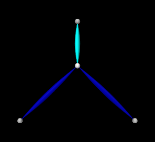
Rendering properties are set at lines 35-38: points are rendered as gray spheres, except for the center particle which is white, and muscles are drawn as spindles, with the exciter muscles blue and the passive target cyan.

Lastly, probes are created: an input probe to specify the target trajectory, an output probe to record target and tracked tensions, and an output probe to record the computed excitations. The first, targetprobe, is attached to the targetForce property of the target component and runs from time 0 to 1 (lines 41-48). Its data is specified in code using addData(), which specifies three knot points with a time step of 0.5. Interpolation set to cubic (line 47) for greater smoothness. The second probe, trackingProbe, records both the target and source tension from the targetForce property of target and the forceNorm property of the passive spring (lines 52-61). The excitation probe is created by the utility method createOutputProbe() supplied by the InverseManager class (lines 64-67, Section 1.4).

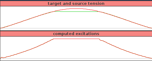
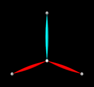
Figure 1.10: Probes showing the combined target and source tension (top) and the computed excitations (bottom) for InverseSpringForce.

To run this example, select All demos > tutorial > InverseSpringForce from the Models menu. The model should load and initially appear as in Figure 1.9 (left). When run, the controller computes excitations to generate the requested tension in the passive spring; this causes the center particle to be pulled down (Figure 1.3, right). Both the target-source and computed excitation probes are shown in Figure 1.10.

For the middle third of the trajectory, the excitation values have reached their threshold value of 1 and so are unable to deliver more force. This in turn causes the source tension (green line) to deviate from the target tension (red line) in the target-source probe.

1.2.8 Target components

As described above, when a motion or force source is added to the controller (using methods such as addPointTarget() or addForceEffectorTarget()), the controller creates and returns a target component that is used for specifying the desired position or force trajectory. Each target term also contains a scalar weight and a vector of subweights, described by the properties weight and subWeights, all of which have default values of 1.0. These weights are used to manage the priorty of the target within the tracking computation; the subWeights vector has a size equal to the number of degrees of freedom (DOF) in the target (3 for points and 6 for frames), and permits fine-grained weighting for each of the targets’s DOFs. The product of the weight with each subweight produces the entries for the diagonal weighting matrix that appears in the various cost terms for motion and force tracking (e.g., ${\bf W}_{m}$ for the motion tracking cost function $\phi_{m}({\bf a})$ in (1.9) and ${\bf W}_{e}$ for the force effector cost function $\phi_{e}({\bf a})$ in (1.11)). Targets (or specific DOFs) with higher weights will be tracked more accurately, while weights of 0 effectively disble tracking.

Target components vary depending on the source component whose position or force is being tracking, but each implements the interface TrackingTarget, which supplies the following methods for controlling the weights and subweights and querying the target’s source component:

ModelComponent getSourceComp()	Returns the target’s source component.
int getTargetSize()	Returns number of target DOFs, which equals the number of subweights.

double getWeight()	Returns the target component weight property.
void setWeight(double w)	Sets the target component weight property.
Vector getSubWeights()	Returns the target component subweights property.
void setSubWeights(VectorNd subw)	Sets the target component subweights property.

1.2.9 Point and frame exciters

In addition to muscle components, exciters may also include PointExciters and FrameExciters, which can be used to apply forces directly to Point or Frame components. This effectively gives the inverse controller the ability to do direct inverse simulation. These exciter components can also assume a role similar to that of the “reserve actuators” used in OpenSim [delp2007opensim], augmenting a model’s tracking capabilities to account for force sources that are not explicitly supplied by the model.

Each exciter applies a force along (or about) a single degree-of-freedom, as specified by the enumerated types PointExciter.ForceDof or FrameExciter.WrenchDof and described in the following table:

Enum field	Description
ForceDof.FX	force along the point x axis
ForceDof.FY	force along the point y axis
ForceDof.FZ	force along the point z axis
WrenchDof.FX	force along the frame x axis (world coordinates)
WrenchDof.FY	force along the frame y axis (world coordinates)
WrenchDof.FZ	force along the frame z axis (world coordinates)
WrenchDof.MX	moment about the frame x axis (world coordinates)
WrenchDof.MY	moment about the frame y axis (world coordinates)
WrenchDof.MZ	moment about the frame z axis (world coordinates)

Point or frame exciters may be created with the following constructors:

PointExciter(Point point, FrameDof dof, double maxForce)	Exciter for point with dof and maxForce.
PointExciter(String name, Point point, FrameDof dof, Mdouble maxForce)	Named exciter for point with dof and maxForce.

FrameExciter(Frame frame, WrenchDof dof, double maxForce)	Exciter for frame with dof and maxForce.
FrameExciter(String name, Frame frame, WrenchDof dof, Mdouble maxForce)	Named exciter for frame with dof and maxForce.

The maxForce argument specifies the maximum force (or moment) that the exciter supplies at an excitation value of 1.0.

If an exciter does not have sufficient strength to facilitate tracking, its excitation value is likely to saturate. This can often be solved by simply increasing the maxForce value.

To allow it to produce negative forces or moments along/about its specified degree of freedom, the excitation bounds for a point or frame exciter must be set to . The TrackingController does this automatically whenever a point or frame exciter is added to it.

For convenience, PointExciter and FrameExciter provide static methods for creating sets of exciters to control all the translational forces and/or moments on a given point or frame:

ArrayList<PointExciter> createPointExciters (MechModel mech, MPoint point, double maxForce, boolean createNames)	Create three exciters to control all forces on a point.

ArrayList<FrameExciter> createFrameExciters ( MMechModel mech, Frame frame, double maxForce, Mdouble maxMoment, boolean createNames)	Create six exciters to control all forces & and moments on a frame.

ArrayList<FrameExciter> createForceExciters (MechModel mech, MFrame frame, double maxForce, boolean createNames)	Create three exciters to control all forces on a frame.

ArrayList<FrameExciter> createMomentExciters ( MMechModel mech, Frame frame, Mdouble maxMoment, boolean createNames)	Create three exciters to control all moments on a frame.

If the (optional) mech argument in these methods is is non-null, the exciters are added to the MechModel’s forceEffectors list. If the argument createNames is true, and the point or frame itself has a non-null name, then the exciter is assigned a name based on the point/frame name and the degree of freedom.

1.2.10 Example: controlling ToyMuscleArm with FrameExciters

The InverseMuscleArm example of Section 1.2.4 can be modified to use frame exciters in place of its muscles, allowing link forces to be controlled directly to make the marker follow the specified path. The modified model is artisynth.demos.tutorial.InverseFrameExcitereArm, and the sections of code where it differs from InverseMuscleArm:sec are listed below:

⬇

27 /**

28 * Creates a frame exciter for a rigid body, controlling the force DOF

29 * described by ’dof’ with a maximum activation for of ’maxf’, and adds it

30 * to both the mech model and the tracking controller ’tcon’.

31 */

32 void addFrameExciter (

33 TrackingController tcon, RigidBody body, WrenchDof dof, double maxf) {

34 FrameExciter fex = new FrameExciter (null, body, dof, maxf);

35 myMech.addForceEffector (fex);

36 tcon.addExciter (fex);

37 }

⬇

48 TrackingController tcon = new TrackingController (myMech, "tcon");

49 addController (tcon);

50 // For each muscle, reinitialize its rest length for the new

51 // configuration

52 for (AxialSpring spr : myMech.axialSprings()) {

53 spr.setRestLength (spr.getLength());

54 }

55 for (MultiPointSpring spr : myMech.multiPointSprings()) {

56 spr.setRestLength (spr.getLength());

57 }

59 // For each link, add two frame exciters to give the controller access to

60 // translational forces in the x-z plane

61 addFrameExciter (tcon, myLink0, WrenchDof.FX, 200);

62 addFrameExciter (tcon, myLink0, WrenchDof.FZ, 200);

63 addFrameExciter (tcon, myLink1, WrenchDof.FX, 200);

64 addFrameExciter (tcon, myLink1, WrenchDof.FZ, 200);

After the controller is created (lines 48-49), the muscle rest lengths are reset, as they are for InverseMuscleArm, but they are not added to controller as exciters. Instead, four frame exciters are created to generate translational forces on each link in the x-z plane, up to a maximum force of 200 (lines 61-64). These exciters are created using the method addFrameExciter() (lines 32-37), which creates the exciter and adds it to the MechModel and to the controller’s exciter list.

Instead of calling the method addFrameExciter(), the frame exciters could have been generated using the following code fragment:

⬇

tcon.addExciters (

FrameExciter.createForceExciters (

myMech, myLink0, 200, /*createNames*/false));

tcon.addExciters (

FrameExciter.createForceExciters (

myMech, myLink1, 200, /*createNames*/false));

This would create six exciters instead of four (three forces per link, instead of limiting forces to x-z plane), but the additional forces would simply not be recruited by the controller.

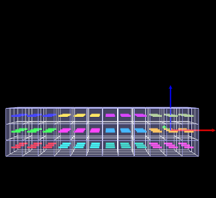
Figure 1.11: Excitations computed for InverseFrameExciterArm.

To run this example, select All demos > tutorial > InverseFrameExciterArm from the Models menu. The excitations generated by running the model are shown in Figure 1.11.

1.3 Tracking controller structure and settings

1.3.1 Controller structure

Figure 1.12: Expanded navigation panel view of the tracking controller (named "tcon") and all its subcomponents, for the example InverseMuscleArm.

The tracking controller is a composite component, which contains the exciter list and the various cost and constraint terms as subcomponents. Some of these components are added as needed. They include the following, as described by their names:

exciters: A list of references to the exciters which have been added to the controller. Note that this is a list of references; the exciters themselves exist elsewhere in the model. Always present.
motionTerm: The MotionTargetTerm detailed in Section 1.2.2.1. Implements the motion cost term $\phi_{m}({\bf a})$ defined in (1.7), and the motion tracker of Figure 1.1. Allocates and maintains target components for motion sources, storing the targets in the subcomponent lists targetPoints and targetFrames, and references to the sources in the reference lists sourcePoints and sourceFrames. Always present.
forceEffectorTerm: The ForceEffectorTerm detailed in Section 1.2.6.1. Implements the force effector cost term $\phi_{e}({\bf a})$ defined in (1.11). Allocates and maintains target components for force effector sources, storing then in the subcomponent list forceTargets. Added on demand.
boundsTerm: Implements the actuator bounds ${\bf a}_{\text{min}}\leq{\bf a}\leq{\bf a}_{\text{max}}$ , where ${\bf a}_{\text{min}}$ and ${\bf a}_{\text{max}}$ are nominally $\bf 0$ and $\bf 1$ . Always present.
L2RegularizationTerm: Implements the cost term for L2 regularization (Section 1.2.3.1). Added on demand.
dampingTerm: Implements the cost term for excitation damping (Section 1.2.3.2). Added on demand.

1.3.2 Controller properties

The controller and its cost terms have a number of properties that can be used to adjust the controller’s behavior. They can be set interactively, either through the inverse controller panel created by the InverseManager (Section 1.4.3), or by selecting the relevant component in the navigation panel and choosing "Edit properties ..." from the context menu. The properties can also be set in code, using the accessor methods supplied by their host component. These methods will usually be named getXxx() and setXxx() for property xxx.Properties of the tracking controller itself include:

active: Controls whether or not the controller is active. Setting this to false turns the controller off. Default value is true.
normalizeCostTerms: Controls whether or not the cost terms are normalized. Normalizing the terms helps ensure that their weights (e.g., $w_{m}$ , $w_{e}$ , and $w_{a}$ in (1.12) more accurately control the tradeoffs between terms. Default value is true.
computeIncrementally: Controls whether excitation values should be computed incrementally, as described in Section 1.1.5. Default value is false.
excitationBounds: Specifies the default excitation bounds for exciter components. Default value is .
targetsVisible: Controls the visibility of the motion target terms contained within the controller, as described in Section 1.2.2.2. Default value is true.
configExcitationColoring: If enabled, automatically configures exciters which support excitation coloring to vary from white to red as their excitation increases (Section 1.2.1.1). Default value is true.
probeDuration: Default duration of probes managed by the InverseManager class (Section 1.4). Default value is 1.0.
probeUpdateInterval: Default update interval of output probes managed by the InverseManager class (Section 1.4). Default value is -1, which means that the interval will default to the simulation step size.
useKKTFactorization: Uses a more computationally expensive but possibly more accurate method to compute the excitation response matrices matrices such as ${\bf H}_{m}$ and ${\bf H}_{e}$ (Section 1.1.3). Default value is false.
maxExcitationJump: Experimental property that limits the change in excitation durig any time step. Default value is false.
useTimestepScaling: Experimental property which enables scaling of all the cost terms by the simulation time step. Default value is false.
debug: Enabled debugging messages. Default value is false.

1.3.3 Motion term properties

The motion target term (Section 1.2.2.1) exports a number of properties that control motion tracking:

enabled: Controls whether or not this term is enabled. Default value is true.
weight: Specifies the weight $w_{m}$ of this term relative to the other cost terms. Default value is 1.0.
chaseTime: Specifies the chase time used for chase control (Section 1.1.2.1). Default value is 0.01.
usePDControl: Controls whether or not PD control is used (Section 1.1.2.2). Default value is false.
Kp: Specifies the proportional terms for PD control (Section 1.1.2.2). Default value is 10000.
Kd: Specifies the derivative terms for PD control (Section 1.1.2.2). Default value is 100.
legacyControl: Controls whether or not legacy control is used. Default value is false.

1.3.4 Properties for other cost terms

All other cost terms, including the L2 regularization (Section 1.2.3.1), export the following properties:

enabled: Controls whether or not the term is enabled. Default value is true.
weight: Specifies the weight of this term relative to the other cost terms. Default value is 1.0.

1.4 Managing probes and control panels

The tracking controller package provides the helper class InverseManager to aid with the creation of probes and control panels that are useful in for inverse simulation applications. The functionality provided by InverseManager is described in this section, and additional documentation may be found in its API documentation.

1.4.1 Inverse simulation probes

ProbeID	I/O type	Probe name	Default filename
TARGET_POSITIONS	input	"target positions"	target_positions.txt
INPUT_EXCITATIONS	input	"input excitations"	input_excitations.txt
TRACKED_POSITIONS	output	"tracked positions"	tracked_positions.txt
SOURCE_POSITIONS	output	"source positions"	source_positions.txt
COMPUTED_EXCITATIONS	output	"computed excitations"	computed_excitations.txt

Table 1.1: Probe types, names, and default file names associated with ProbeID.

InverseManager contains static methods that support the creation and management of a variety of probes related to inverse simulation. These probes are defined by the enumerated type InverseManager.ProbeID, which includes the following identifiers:

TARGET_POSITIONS: An input probe which provides a trajectory ${\bf x}_{t}(t)$ for all motion targets. Its input values are attached to the position property (3 values) of each point target and the position and orientation properties of each frame target (7 values), in the order the targets appear in the controller.
INPUT_EXCITATIONS: An input probe which provides input excitation values for all the controller’s exciters, in the order they appear in the controller. This probe can be used for testing purposes, in order to see what trajectory can be expected to arise from a given excitation input.
TRACKED_POSITIONS: An output probe which records the positions of all motion targets as they are set by the controller. Its output values are extracted from the same component properties used by TARGET_POSITIONS.
SOURCE_POSITIONS: An output probe which records that actual position tracjectory ${\bf x}(t)$ followed by all motion souces. Its output values are extracted from the same component properties used by TARGET_POSITIONS.
INPUT_EXCITATIONS: An output probe which records the computed excitation values for all the controller’s exciters, in the order they appear in the controller.

Each of these probes is associated with both a name and a default file name (Table 1.1), where the default file name may be assigned if another file path is not explcitly specified.

When a default file name is used, it is assumed to be relative to the ArtiSynth working folder, as described in Section LABEL:Probes:sec.

These probes may be created, for a given tracking controller, with the following (static) InverseManager methods:

NumericInputProbe createInputProbe (TrackingController tcon MProbeID pid, String filePath, double start, double stop)	Create input probe specified by pid.

NumericOutputProbe createOutputProbe (TrackingController tcon MProbeID pid, String filePath, double start, double stop, Mdouble interval)	Create output probe specified by pid.

Here pid specifies the probe type, filePath an (optional) file path, start and stop the start and stop times, and interval the output probe update interval. Input probes are initialzed to use Interpolation.Order#CubicStep interpolation.

Created probes may be added to the application root model as needed.

Most of the examples above use createOutputProbe() to create a computed excitations probe. In InverseMuscleFem (Section 1.2.5), the two output probes used to display the tracked position and orientation of myFrame, created at lines (42-51), could be replaced by a single probe of type SOURCE_POSITIONS, using a code fragment like this:

⬇

NumericOutputProbe sourceProbe = InverseManager.createOutputProbe (

tcon, ProbeID.SOURCE_POSITIONS, /*fileName=*/null,

startTime, stopTime, /*interval=*/-1);

addOutputProbe (sourceProbe);

Likewise, a probe showing the target position and orientation, for purposes of comparing it against SOURCE_POSITIONS and evaluating the tracking error, could be created using

⬇

NumericOutputProbe trackedProbe = InverseManager.createOutputProbe (

tcon, ProbeID.TRACKED_POSITIONS, /*fileName=*/null,

startTime, stopTime, /*interval=*/-1);

addOutputProbe (trackedProbe);

For both these method calls, the source and target components (myFrame and target in the example) are automatically located within the tracking controller.

One reason to create a TRACKED_POSITIONS probe, instead of comparing SOURCE_POSITIONS directly against the trajectory input probe, is that the former is guaranteed to have the same number of data points as SOURCE_POSITIONS, whereas a trajectory probe, being an input probe, may not. Moreover, if the trajectory is being produced using a controller, a trajectory probe may not even exist.

For convenience, InverseManager also provides methods to add a complete set of default probes to the root model:

void addProbes (RootModel root, TrackingController tcon, Mdouble duration, double interval)	Add default probes to root.

void resetProbes (RootModel root, TrackingController tcon, Mdouble duration, double interval)	Clear probes and add default probes to root.

addProbes() creates a COMPUTED_EXCITATIONS probe and an INPUT_EXCITATIONS probe, with the latter deactivated by default. If the controller has any motion targets, it will also create TARGET_POSITIONS, TRACKED_POSITIONS and SOURCE_POSITIONS probes. Probe start times are set to 0, stop times are set to duration, and the output probe update interval is set to interval, with -1 causing the interval to default to the simulation step size. Probe file names are set to the default file names described in Table 1.1. Since these file names are relative, the files themselves are assumed to exist in the ArtiSynth working folder, as described in Section LABEL:Probes:sec. Input probes are initialzed to use Interpolation.Order#CubicStep interpolation. If the file for an input probe actually exists, it is used to initialize the probe’s data; otherwise, the probe data is initialized to 0 and the probe is deactivated.

resetProbes() removes all existing probes and then behaves identically to addProbes().

InverseManager also supplies methods to locate and adjust the probes that it has created:

NumericInputProbe findInputProbe (RootModel root, ProbeID pid)	Find specified input probe.
NumericOutputProbe findOutputProbe (RootModel root, ProbeID pid)	Find specified output probe.
Probe findProbe (RootModel root, ProbeID pid)	Find specified input or output probe.

boolean setInputProbeData (RootModel root, MProbeID pid, double[] data, double timeStep)	Set input probe data.

boolean setProbeFileName (RootModel root, MProbeID pid, String filePath)	Set probe file path.

The findProbe() methods search for the probe specified by pid within a root model, using the probe’s file name (Table 1.1) as a search key. The method setInputProbeData() searches for a specified probe, and if it is found, sets its data using the probe’s setData(double[],double) method and returns true. Likewise, setProbeFileName() searches for a specified probe and sets its file path.

Since probes maintained by InverseManager use probe names as a search key, care should be taken to ensure that these names do not conflict with those of other application probes.

1.4.2 Example: using InverseManager probes

The example InverseMuscleArm (Section 1.2.4) has been configured for use with the InverseManager by setting its working folder to inverseMuscleArm located beneath its source folder. If instead of creating the target and output excitations probes (lines 34-52), addProbes() is simply called at the end of the build() method (after the working folder has been set), as in

⬇

// set working folder for probe files

ArtisynthPath.setWorkingFolder (

new File (PathFinder.getSourceRelativePath (this, "inverseMuscleArm")));

InverseManager.addProbes (this, tcon, 5.0, -1);

then a set of probes will be created as shown in Figure 1.13. The tracing probes ("target tracing" and "source tracing") are still present, in addition to five default probes. TARGET_POSTIONS and INPUT_EXCITATIONS are expanded to show the data that has been automatically loaded from the files target_positions.txt and input_excitations.txt located in the working folder. By default, the former probe is enabled and the latter is disabled. If the model is run, inverse simulation will proceed as before.

Figure 1.13: InverseMuscleArm probes with original tracing probes and default probes.

After loading the probes, the application could disable the tracking controller and enable the input excitations:

⬇

// set working folder for probe files

ArtisynthPath.setWorkingFolder (

new File (PathFinder.getSourceRelativePath (this, "inverseMuscleArm")));

InverseManager.addProbes (this, tcon, 5.0, -1);

tcon.setActive (false);

InverseManager.findProbe (this, ProbeID.INPUT_EXCITATIONS).setActive (true);

This will cause the simulation to run “open loop” in response to the excitations. However, because the input excitations are slightly different than those that were computed by the controller, there is a now a considerable tracking error (Figure 1.14, left).

After the open loop run, one can save the resulting SOURCE_POSITIONS probe, which will write the file "target_positions.txt'' into the working folder. This can then be used to generate a new target trajectory, by copying it to "target_positions.txt". If the model is reloaded, the new trajectory will now appear in the TARGET_POSITIONS probe (Figure 1.15). Deactivating the INPUT_EXCITATIONS probe and reactivating the tracking contoller will cause this new trajectoty to be tracked properly (Figure 1.14, right).

In ways such as this, the probes may be used to examine the behavior and performance of the tracking controller.

Figure 1.14: Left: InverseMuscleFem when run open loop with excitations loaded from "input_excitations.txt". Right: model run with inverse simulation, using new targets generated by the open loop run.

Figure 1.15: InverseMuscleArm probes with new target trajectory copied from the open loop run.

1.4.3 Inverse control panel

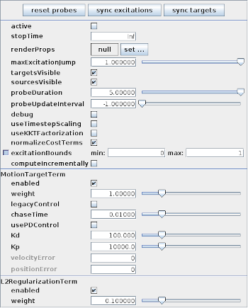
InverseManager also provide methods to create and manage an inverse control panel, which allows interactive editing of the properties of the tracking controller and its various cost terms, as described in Section 1.3. Applications can create an instance of this panel in their build() method, as the InverseMuscleArm example (Section 1.2.4) does at line 65:

⬇

InverseManager.addInversePanel (this, tcon);

The panel is automatically configured to display the properties of the cost terms with which the controller is currently configured. Figure 1.16 shows the panel for InverseManager.

Figure 1.16: Inverse control panel created for the InverseMuscleArm demo.

The following methods are supplied by InverseManager() to manage inverse control panels:

ControlPanel createInversePanel (TrackingController tcon)	Create inverse control panel for tcon.
ControlPanel createInversePanel (RootModel root, MTrackingController tcon)	Create and add inverse control panel to root.
ControlPanel findInversePanel (RootModel root)	Find inverse control panel in root.

At the top of the inverse panel are three buttons: "reset probes", "sync excitations", and "sync targets". The first uses InverseManager.resetProbes() to clear all probes and recreate the default probes, using the duration and update interval specified by the tracking controller properties probeDuration and probeUpdateInterval. The second button copies the contents of the COMPUTED_EXCITATIONS probe into the INPUT_EXCITATIONS probe. If this is done after excitations have been computed, then running the simulation again with the controller deactived and INPUT_EXCITATIONS activated should produce an identical motion. The third button copies the contents of the SOURCE_POSITIONS probe into the TARGET_POSITIONS. This can be used to verify that a source trajectory created open loop with a prescribed set of input excitations can in fact be tracked by the controller.

The probe copy methods used by the “sync” buttons are also available to the application code:

boolean syncTargetProbes (RootModel root)	Copy SOURCE_POSITIONS into TARGET_POSITIONS.
boolean syncExcitationProbes (RootModel root)	Copy COMPUTED_EXCITATIONS into INPUT_EXCITATIONS.

1.5 Caveats and limitations

Use of the inverse controller is subject to some caveats.

•

Tracked components must be dynamic, in that their motion is controlled by forces. This means that their dynamic property must be set to true or they must be attached to other bodies that are dynamic.
•

The algorithm which computes the excitations currently has a complexity $O(n^{3})$ in the number of excitations . This is due both to the use of numeric differentation for determining excitation response matrices such as ${\bf H}_{m}$ and ${\bf H}_{e}$ (Section 1.1.3), and also the fact that the QP solver is at present a dense solver. This means that applications with large numbers of excitations may require considerably longer to simulate than those with fewer excitations.
•

The controller is not designed to work with unilateral constraints (the most common examples of which are constraint-based contact and joint limits). For models containing these behaviors, inverse simulation may produce excitations that jump around erratically. In the case of collisions, one solution may be to use force-based collisions, implemented with either PointPlaneForce or PointMeshForce, as described in Section LABEL:OtherPointForces:sec. Setting these components to use a quadratic force function may improve performace even more. Another possible solution, for any kind of unilateral constraint, may be to make it compliant (Sections LABEL:JointCompliance:sec and LABEL:ContactRegularization:sec), since this has the same effect as making the constraint force-based.
•

Prescribed motion trajectories may need to be sufficiently smooth the avoid large transient excitations, particularly at the start and end of motions when velocities transition from and to 0. Transient effects are often more pronounced for models where inertial effects are high. Cubic interpolation is useful for creating smoother trajectories, particularly with a limited number of data points. It may also be necessary to expliclty smooth an input trajectory with additional points.

In the InverseMuscleArm example, there is a noticable transient at the start (Figure 1.6, left). Increasing the L2 regularization weight reduces the transient amplitude but spreads it out over a longer time (Figure 1.6, right), at the expense of tracking accuracy.

Generated on Wed Jul 17 20:30:54 2024 by LaTeXML [LOGO]

Inverse Simulation

Contents

Chapter 1 Inverse Simulation

1.1 Overview

1.1.1 Tracking controller operation

1.1.2 Motion tracking

1.1.2.1 Chase control

1.1.2.2 PD control

1.1.3 Generating excitations using a quadratic program

1.1.4 Force tracking

1.1.5 Incremental computation

1.1.6 Setting up the tracking controller

1.1.7 Example: moving a point with multiple Muscles

1.2 Tracking controller components

1.2.1 Exciters

1.2.1.1 Excitation coloring

1.2.2 Motion targets

1.2.2.1 Motion target term

1.2.2.2 Motion target rendering

1.2.3 Regularization

1.2.3.1 L2 Regularization

1.2.3.2 Excitation damping

1.2.4 Example: controlling ToyMuscleArm

1.2.5 Example: controlling an FEM muscle model

1.2.6 Force effector targets

1.2.6.1 Force effector term

1.2.7 Example: controlling tension in a spring

1.2.8 Target components

1.2.9 Point and frame exciters

1.2.10 Example: controlling ToyMuscleArm with FrameExciters

1.3 Tracking controller structure and settings

1.3.1 Controller structure

1.3.2 Controller properties

1.3.3 Motion term properties

1.3.4 Properties for other cost terms

1.4 Managing probes and control panels

1.4.1 Inverse simulation probes

1.4.2 Example: using InverseManager probes

1.4.3 Inverse control panel

1.5 Caveats and limitations