7 The Timeline
The timeline is a panel that provides “play” controls for starting and stopping the simulation, and allows the user to graphically arrange temporal sequences of probes and waypoints to control and monitor the simulation. If not initially visible, its visibility can be toggled by hitting the ‘t’ key from within the viewer (Section 3.12).
7.1 Probes and waypoints
ArtiSynth allows models to connect to special components, known as probes, which can either supply input values or monitor output values over time as the simulation proceeds. Probes attached to simulation inputs are known as input probes (class InputProbe), while those attached to outputs are known as output probes (class OutputProbe). Each probe has a start time and a stop time, and implements an apply(t0,t1) method that supplies (or collects) data for the simulation step between time t0 and t1. Probes are described in more detail, along with specifics about how to code them into applications, in the “Simulation Control” chapter of the ArtiSynth Modeling Guide.
The most commonly used probe subclasses are NumericInputProbe and NumericOutputProbe, each of which is associated with a vector of floating point values that are interpolated over time. This data is usually connected to various model component properties, and used to either set (for input probes) or collect (for output probes) the values of those properties. The size of the vector is known as the probe’s vector size and matches the properties that the probe is connected to. For example, a probe controlling a single muscle excitation value will have a vector size of one, whereas a probe collecting the 3D velocity of a point will have a vector size of three.
Within a numeric probe, data is defined by a temporal sequence of knots points which give the vector values at prescribed times, with values in between determined by interpolation (Section 7.5.7). For input probes, the knot density is often sparse, whereas for output probes it matches the sample rate at which data is collected, which is usually the simulation step size.
Input and output probes are arranged and displayed graphically in the timeline, within a set of tracks (Section 7.4). Each probe is displayed as a bar within one of these tracks. The display for numeric probes can also be expanded to show a graph of the numeric data (Section 7.5).
ArtiSynth allows models to set temporal waypoints, which are designated times at which the model state is saved during simulation. This allows the simulation to be later reset to that time without having to recompute the simulation from the beginning. A special type of waypoint is known as a breakpoint, which causes the simulation to pause when it is reached. The timeline displays the waypoints, and allows them to be created and edited (Section 7.3).
7.2 Basic timeline structure
The basic structure of the timeline is shown in Figure 31.
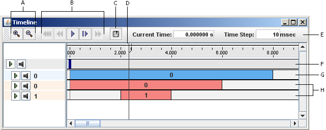
The toolbar at the top contains the following widgets:
- Zoom controls
-
Shrinks or expands the timescale.
- Play controls
-
Starts, pauses, or resets the simulation.
- Save button
-
Saves the data for all output probes with attached files.
- Time box
-
Shows the current simulation time.
- Time step box
-
Shows the length of time associated with a “single step” command.
7.2.1 Play controls
The play controls are in turn comprised of the following buttons:
| Reset: | Resets the simulation to the beginning at time 0. | |
| Skip-back: | Moves the simulation time backward to the previous valid waypoint (see Section 7.3). | |
| Play: | Starts the simulation. | |
| Pause: | Takes the place of the play button and pauses the simulation. | |
| Single-step: | Advances the simulation by a single step, specified in the time step box. | |
| Skip-forward: | Moves the simulation time forward to the next valid waypoint (see Section 7.3). | |
| Stop-all: | Stops the simulation and any currently running Jython commands and scripts (Section 12.3). |
7.2.2 Tracks
The timeline proper is divided into a number of tracks. At the top is the waypoint track, which is used to arrange waypoints and breakpoints. Below that are a variable number of input and output tracks, which are used respectively for arranging the input and output probes.
7.3 Viewing and setting waypoints
7.3.1 Waypoints
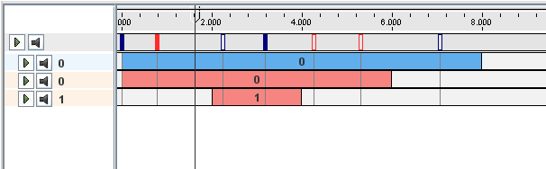
Waypoints are arranged along the waypoint track at the top of the timeline and are indicated by a small rectangular blue box (Figure 32). A solid box indicates a waypoint that contains a valid state and thus can be advanced to using the fast forward/backward buttons.
To add a waypoint, right-click on the waypoint track. A popup menu will show a number of options, including Add waypoint here, which adds a waypoint at the current location of the time cursor, and Add waypoint(s), which will bring up a dialog prompting for a specific time to add a Waypoint. The "Add Waypoint" dialog also contains a repeat field, which will cause additional waypoints to be added with a spacing indicated by the time value, and an option to create breakpoints instead of waypoints.
Once created, waypoints can be moved by dragging them. They can also be deleted by right-clicking on them and selecting the Delete waypoint option.
To delete all the waypoints, select Delete waypoints, either from the main File menu, or after right-clicking on the waypoint track.
7.3.2 Breakpoints
Breakpoints are waypoints that also cause the simulation to stop. They are displayed in red instead of blue.
Breakpoints can be added in the same way as waypoints, i.e., by right clicking on the waypoint track and selecting Add breakpoint here or Add waypoint(s).
Waypoints can be converted into breakpoints (and vice versa) through the context menu.
7.3.3 Saving and loading
It is possible to save and load waypoints to and from an external file. The following menu options may be selected to do this, either from the main File menu, or after right-clicking on the waypoint track:
- Save waypoints as ...
-
Brings up a file chooser that allows the user to specify a file for saving all waypoints and their state data. Clicking Save As completes the operation.
- Save waypoints
-
If a waypoint file has already been specified using either “Save waypoints as ...” or “Load waypoints ...”, then all waypoints and their state data are saved to that file.
- Load waypoints ...
-
Brings up a file chooser that allows the user to specify a file from which waypoints and their state data will be loaded. Clicking Load completes the operation. The new waypoints are added to any existing ones, but previously waypoints are not deleted. Checks are made to help ensure that the waypoint data is consistent with the model’s current state.
- Reload waypoints
-
Identical to “Load waypoints ...”, except that it uses a file that has already been specified using either “Save waypoints as ...” or “Load waypoints ...”.
- Delete waypoints
-
Deletes all waypoints except the one at time zero.
Waypoint files are currently stored as binary files. The reason for this is that the required storage is about 1/2 of that required for text files, while the writing and parsing times are as much as
faster.
7.4 Tracks and probes
Probes are arranged on tracks located beneath the waypoint track. Input probes must be placed on input tracks and output probes must be placed on output tracks. Furthermore, probes on the same track are not allowed to overlap.
Note:
In the future, additional restrictions may be placed on what type of probe can be placed on what track.
Probes can be moved horizontally to different times as well as vertically onto different tracks. They can also be stretched by dragging the edges of the probe and cropped by holding the control key while stretching.
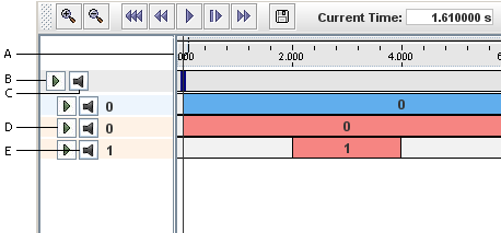
On the left side of the timeline is the track panel, which contains a number of track control widgets (Figure 33).
7.4.1 Creating, moving, and deleting tracks
New tracks may be added by right-clicking in the waypoint track and selecting Add input track or Add output track.
The vertical location of a track can be moved by left clicking on it in the left panel and dragging it up or down to a new location.
A track can be deleted by right-clicking on the track in the track panel and selecting Delete track.
7.4.2 Muting tracks
A track can be muted or unmuted by clicking on its gray mute button in the track panel (Figure 33). All probes on a muted track are ignored during simulation.
All tracks can be muted, thus disabling all probes, by clicking on the mute all button in the gray panel above the tracks.
7.4.3 Expanding tracks
A track can be expanded or collapsed by clicking on its green expand button in the track panel (Figure 33). Expanding a track creates an additional area in which the data associated with the track’s probes may be displayed (see Figure 34). The way in which this data is displayed is probe-specific. Probes containing numeric data usually show their data graphically, as described in Section 7.5.
7.4.4 Grouping tracks
Multiple contiguous tracks can be selected by clicking on them while holding the control key. Furthermore, they can be grouped together or ungrouped by selecting the appropriate option from the context menu. Grouped tracks can be collapsed, moved simultaneously and muted together.
7.5 Numeric probe displays
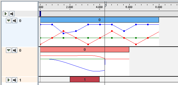
Data associated with numeric probes is displayed as a graph within the display (Figure 34), with each entry in a probe’s data vector drawn as a separate trace. If the probe’s vector size is greater than one, each trace is drawn using a different color (up to a limit, after which colors are reused).
7.5.1 Setting the range and display properties
The range and other properties of the display can be set by right clicking in the display and selecting “Edit range and properties ...”, which creates a dialog that allows these to be adjusted. If the autoRanging property is set to true, then the display range automatically expands as needed to accommodate new data. Display ranges can also be adjusted to fit the current data by right-clicking in the display and selecting Fit ranges to data.
Large data displays (Section 7.5.2) contain additional GUI-based features to adjust the display range.
7.5.2 Large displays
A large display for a numeric probe can be created by right-clicking on the probe icon and selecting Large Display. This will create a large numeric display in a separate panel, allowing more precise inspection of data (Figure 35).
In addition to the functionality of the smaller displays, large displays have additional buttons, located across the top, for controlling the display range and other items. The first four of these are mode buttons:
| Select: | Places the display into selection mode, allowing knots (when visible) to be edited as described in Section 7.5.5. | |
| Zoom in: | Places the display into zoom in mode, in which the user can zoom in by either drag-selecting a region, or by left clicking on a point of interest. The mouse wheel can also be used to zoom in or out. | |
|
|
Zoom out: | Places the display into zoom out mode, in which the user can zoom out by left clicking on a point of interest. The mouse wheel can be also used to zoom in or out. |
|
|
Translate: | Places the display into translate mode, in which the user can translate a (zoomed-in) display using the left mouse button. The mouse wheel can also be used to zoom in or out. |
There are also several additional buttons:
| Increase y: | Increases the vertical y range. | |
| Decrease y: | Decreases the vertical y range. | |
| Decrease x: | Decreases the horizontal x range. | |
| Increase x: | Increases the horizontal x range. | |
| Fit Range: | Fits the vertical and horizontal ranges to the current data. | |
| Grid: | Enables or disables visibility of a grid that aligns with the x and y axis tick marks. | |
| Auto range: | Enables or disables auto-ranging, in which the y axis is automatically adjusted to fit new data. |
7.5.3 Cloning displays and exporting plots
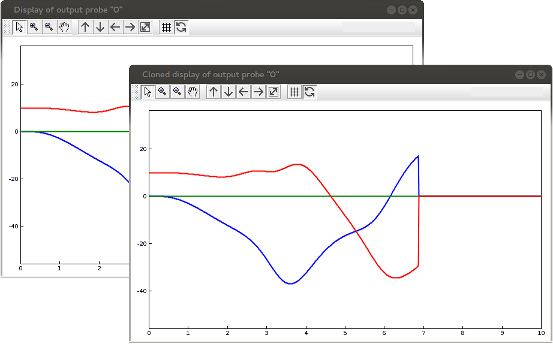
Large data displays can be cloned by right-clicking in the display and selecting Clone display. This creates a duplicate display (Figure 36) containing a copy of all the data currently in the probe. However, the duplicate display is not attached to the probe, and so the data does not change when the probe is reset or additional data is added to the probe. This is useful for comparing outputs between different simulations.
In addition, it is possible to export a large display’s plot to an image file. Right-click in the display, choose “Export image as ...”, and enter the desired file name and file type in the chooser. The file’s type is indicated by its extension. A range of image file types are supported, including JPEG (.jpg, .jpeg), PNG (.png), scalable vector graphics (.svg), and encapsulated PostScript (.eps).
7.5.4 Legends and visibility control
As mentioned above, each entry in a numeric probe’s data vector is rendered in a different color (up to a limit, currently 30, after which colors are reused). If the vector size is large (say more than three or four), or if there is much overlapping of values, then the result can be difficult to visualize.
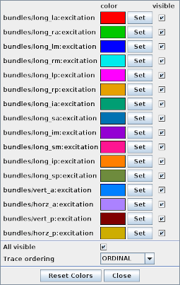
To manage this problem, numeric displays provide a legend dialog that allows the user to control the color, drawing order, and visibility for each vector entry (Figure 37).
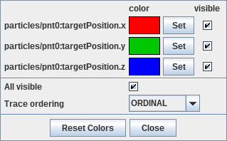
To open the legend dialog, right-click in the display panel and select Show legend. Each row in the legend dialog is associated with a specific trace, consisting of a descriptive label followed by the trace color and a toggle controlling its visibility. For traces associated with component properties, the label consists of a partial path identifying the property, and for vector-valued properties this is followed by the name or number of the corresponding vector element. Traces are rendered in bottom-to-top order, so those at the top will be most visible.
-
•
To change a trace’s color, click the Set button, which will bring up a color menu.
-
•
To make an trace visible or invisible, use the visible toggle box.
-
•
To make all traces visible or invisible, use the All visible toggle box at the bottom of the dialog.
-
•
To change the order in which a trace is drawn, click and drag its dialog entry vertically.
Traces can also be reordered using the Trace ordering selector at the dialog bottom. At the time of this writing, the available orderings include:
- ORDINAL
-
Traces are ordered by their natural place in the probe data. This is the default.
- RMS
-
Traces are ordered in descending order by the RMS (root mean square) of their values over time.
- RANGE
-
Traces are ordered in decreasing order by the difference between their maximum and minimum values over time.
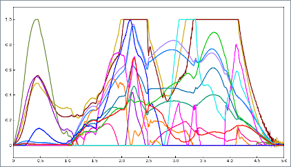
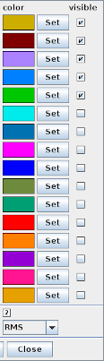
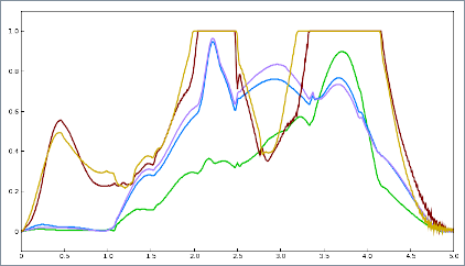
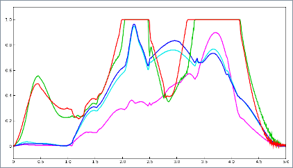
Reordering traces, and then restricting visibility to a few at the top, can allow visualization of the most prominent data in an otherwise crowded display. For example, Figure 38 shows the 16 muscle excitations produced by inverse simulation of a muscular hydrostat model, with the legend dialog shown in Figure 39 (left). To view only the five excitations with the largest RMS values, one can use the Trace ordering selector to sort them in decreasing RMS order, and then make all traces invisible except the top five. The resulting display is shown in Figure 40, with the corresponding legend dialog shown in Figure 39 (middle).
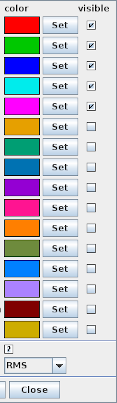
When traces are reordered, their colors are not changed. To reassign the default colors to the traces based on their current ordering, one may use the Reset Colors button at the bottom of the legend dialog. Figure 41 shows the result of doing this for the display of Figure 40, with the corresponding legend dialog shown in Figure 39 (right).
 |
 |
 |
7.5.5 Editing and scaling data
As mentioned in Section 7.1, numeric probe data is described by a temporal sequence of knots, between which data is interpolated as described in Section 7.5.7.
Knot points can be made visible or invisible by setting the display’s knotsVisible property. This can also be done by right-clicking in the display and selecting Show knot points or Hide knot points. The rendered size of the knot, in pixels, is controlled by the knotSize property.
Since output probes typically have a very high knot density, their knots are set to be invisible by default.
For input probes, knot points (when visible) can be edited by moving, adding, or deleting them:
-
•
To move a knot point, left click on the knot and drag it.
-
•
To add a knot point, place the mouse at the desired location and double left-click.
-
•
To delete a knot point, right-click on the knot and select Delete knot point.
-
•
To edit a knot point data value, right-click on the knot and select Edit knot point.
The data for all numeric probes (input or output) can be scaled by right-clicking in the display and selecting “Scale data ...”. This allows the user to enter a scaling factor that is applied uniformly to all the knot points.
7.5.6 Smoothing data
Numeric probe data can also be smoothed, which is convenient for removing noise from either input or output data. To apply data smoothing, right click in the display and select “Smooth data ...”; this will open a smoothing dialog as shown in Figure 42.
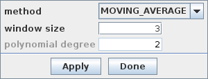
Different smoothing methods are available and can be selected using the dialog’s method field. At the time of this writing, the following methods are available:
- MOVING_AVERAGE
-
Applies a mean average filter across the knots, using a moving window whose size is specified by the window size field. The window is centered on each knot, and is reduced in size near the end knots to ensure a symmetric fit. The end knot values are not changed. The window size must be odd and the window size field enforces this.
- SAVITZKY_GOLAY
-
Applies Savitzky-Golay smoothing across the knots, using a moving window of size
 . Savitzky-Golay smoothing works by fitting the
data values in the window to a polynomial of a specified degree
. Savitzky-Golay smoothing works by fitting the
data values in the window to a polynomial of a specified degree  , and
using this to recompute the value in the middle of the window. The
polynomial is also used to interpolate the first and last
, and
using this to recompute the value in the middle of the window. The
polynomial is also used to interpolate the first and last  values, since it is not possible to center the window on these.
The window size
and the polynomial degree are specified by the
window size and polynomial degree fields. must be odd,
and must also be larger than , and the fields enforce these
constraints.
Note that smoothing makes no adjustment to account for uneven knot spacing, which may sometimes occur for input data.
7.5.7 Interpolation control
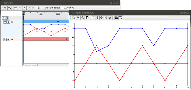
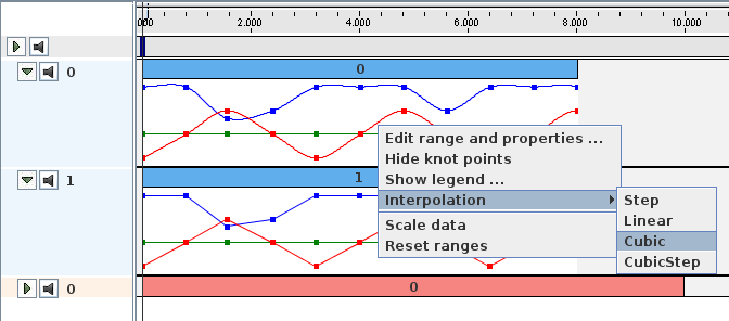
The data between knot points in a numeric probe is interpolated, using one of the interpolation orders described below, with the default interpolation order being Linear. Linear interpolation is almost always sufficient for output probes, which typically have a close spacing between knots that equals the simulation step size. Input probes, on the other hand, often have a much sparser knot spacing and so different interpolation orders can be useful. The interpolation order of input probes can be set by right-clicking in the display and selecting the Interpolation menu item. This is illustrated in Figure 43, which shows two input probes, one using Cubic interpolation and the other using Linear interpolation.
The interpolation options for a numeric probe include:
- Step
-
Values are set to the values of the closest previous knots points.
- Linear
-
Values are set by linear interpolation of the closest surrounding knot points.
- Cubic
-
Values are set by cubic Catmull interpolation between the surrounding knot points.
- CubicStep
-
Values are set by cubic Hermite interpolation between the surrounding knot points, with the slopes at knot points set to zero.
- SphericalLinear
-
When interpolating quaternions or
 rigid transformation
matrices, 3D rotation values are set by piecewise spherical linear
interpolation (i.e., "slerp", as described by Shoemake’s 1985 SIGGRAPH
paper). Otherwise, interpolation is linear. Quaternions are assumed
if the vector size of the numeric probe is 4, and rigid
transformation matrices are assumed if the vector size is 16.
rigid transformation
matrices, 3D rotation values are set by piecewise spherical linear
interpolation (i.e., "slerp", as described by Shoemake’s 1985 SIGGRAPH
paper). Otherwise, interpolation is linear. Quaternions are assumed
if the vector size of the numeric probe is 4, and rigid
transformation matrices are assumed if the vector size is 16. - SphericalCubic
-
When interpolating quaternions or
rigid transformation
matrices, 3D rotation values are set by spherical cubic interpolation
(i.e., "slerp", as described by Shoemake’s 1985 SIGGRAPH paper).
Otherwise, interpolation is cubic. Quaternions are assumed if the
vector size of the numeric probe is 4, and rigid
transformation matrices are assumed if the vector size is 16.
All of the above interpolation orders are instances of the enumeration type Interpolation.Order.
![[LOGO]](data:image/png;base64,iVBORw0KGgoAAAANSUhEUgAAAAsAAAAOCAYAAAD5YeaVAAAAAXNSR0IArs4c6QAAAAZiS0dEAP8A/wD/oL2nkwAAAAlwSFlzAAALEwAACxMBAJqcGAAAAAd0SU1FB9wKExQZLWTEaOUAAAAddEVYdENvbW1lbnQAQ3JlYXRlZCB3aXRoIFRoZSBHSU1Q72QlbgAAAdpJREFUKM9tkL+L2nAARz9fPZNCKFapUn8kyI0e4iRHSR1Kb8ng0lJw6FYHFwv2LwhOpcWxTjeUunYqOmqd6hEoRDhtDWdA8ApRYsSUCDHNt5ul13vz4w0vWCgUnnEc975arX6ORqN3VqtVZbfbTQC4uEHANM3jSqXymFI6yWazP2KxWAXAL9zCUa1Wy2tXVxheKA9YNoR8Pt+aTqe4FVVVvz05O6MBhqUIBGk8Hn8HAOVy+T+XLJfLS4ZhTiRJgqIoVBRFIoric47jPnmeB1mW/9rr9ZpSSn3Lsmir1fJZlqWlUonKsvwWwD8ymc/nXwVBeLjf7xEKhdBut9Hr9WgmkyGEkJwsy5eHG5vN5g0AKIoCAEgkEkin0wQAfN9/cXPdheu6P33fBwB4ngcAcByHJpPJl+fn54mD3Gg0NrquXxeLRQAAwzAYj8cwTZPwPH9/sVg8PXweDAauqqr2cDjEer1GJBLBZDJBs9mE4zjwfZ85lAGg2+06hmGgXq+j3+/DsixYlgVN03a9Xu8jgCNCyIegIAgx13Vfd7vdu+FweG8YRkjXdWy329+dTgeSJD3ieZ7RNO0VAXAPwDEAO5VKndi2fWrb9jWl9Esul6PZbDY9Go1OZ7PZ9z/lyuD3OozU2wAAAABJRU5ErkJggg==)