10 Inverse Simulation 10 Inverse Simulation 10.2 Tracking controller components

10.1 Overview

ArtiSynth supports an inverse simulation capability that allows the computation of the excitation signals (for muscles and other actuators) needed to track target trajectories for a set of source components within the model (typically points or frames). This is achieved using a specialized controller component known as a TrackingController, defined in the package

  artisynth.core.inverse

An application model creates the tracking controller and configures it with the source components, the exciter components needed to effect the tracking, and probes or controllers to specify the target trajectories. Then at each simulation time step the controller computes the excitations (i.e., signals to the exciter components) that allow the trajectories to be followed as closely as possible, in a manner conceptually similar to computed muscle control in OpenSim [7].

It is currently recommended to run inverse simulation with hybrid solving disabled. Hybrid solving combines direct and iterative solution techniques to speed up sparse matrix solves within ArtiSynth’s integrators. However, it can occasionally cause stability issues when used with inverse control. Hybrid solves can be disabled in several ways:
1.

By setting hybridSolvesEnabled to false under “Settings > Simulation ...” in the GUI; see “Simulation” under “Settings and Preferences” in the ArtiSynth User Interface Guide. This change can be made to persist across ArtiSynth restarts.
2.
By calling the static method setHybridSolvesEnabled() of MechSystemSolver in the model’s build() method:
   MechSystemSolver.setHybridSolvesEnabled(false);

10.1.1 Tracking controller operation

Let ${\bf q}$ , ${\bf u}$ and ${\bf f}$ be composite vectors describing the positions, velocities and forces of all the components in the application model, and let ${\bf a}$ be a vector of excitation signals for all the excitation components available to the controller. ${\bf f}$ can be decomposed into

${\bf f}={\bf f}_{p}({\bf q},{\bf u})+{\bf f}_{a}({\bf q},{\bf u},{\bf a})$

(10.1)

where ${\bf f}_{p}$ are the passive forces corresponding to zero excitation, and ${\bf f}_{a}$ are the active forces. During simulation, the controller computes values for ${\bf a}$ to best track the target trajectories.

In the case of motion tracking, let ${\bf x}$ and ${\bf v}$ be the subvectors of ${\bf q}$ and ${\bf u}$ containing the positions and velocities of the source components, and let ${\bf x}_{t}$ and ${\bf v}_{t}$ be the corresponding target trajectories. At the beginning of each time step, the controller compares the current source velocity state $({\bf x},{\bf v})$ with the desired target state $({\bf x}_{t},{\bf v}_{t})$ and uses this to determine a desired source velocity ${\bf v}_{*}$ for the next time step; this computation is done by the motion tracker (Figure 10.1, Section 10.1.2). An excitation generator then computes ${\bf a}$ in order to try and make ${\bf v}$ match ${\bf v}_{*}$ (Section 10.1.3).

The excitation generator accepts a desired velocity ${\bf v}_{*}$ instead of a desired acceleration because ArtiSynth’s physics engine computes velocity changes directly.

Figure 10.1: Tracking controller operation for motion targets.

10.1.2 Motion tracking

As mentioned above, the motion tracker computes a desired source velocity ${\bf v}_{*}$ for the next time step based on the current source state $({\bf x},{\bf v})$ and desired target state $({\bf x}_{t},{\bf v}_{t})$ . This can be done in two ways: chase control (the default), and PD control.

10.1.2.1 Chase control

Chase control simply sets ${\bf v}_{*}$ to ${\bf v}_{t}$ , plus an additional velocity that tries to reduce the position error ${\bf x}_{t}-{\bf x}$ over a specified time interval , called the chase time:

${\bf v}_{*}={\bf v}_{t}+\frac{{\bf x}_{t}-{\bf x}}{T}.$

(10.2)

In general, should be greater than or equal to the simulation step size . If it is greater, then ${\bf x}$ will tend to lag behind ${\bf x}_{t}$ , but this will also reduce the potential for overshoot due to system nonlinearities. Conversely, if if less than , then ${\bf x}$ is much more likely to overshoot. The default value of is 0.01.

10.1.2.2 PD control

PD control computes a desired source acceleration $\dot{\bf v}_{*}$ based on

$\dot{\bf v}_{*}=K_{p}({\bf x}_{t}-{\bf x})+K_{d}({\bf v}_{t}-{\bf v}),$

(10.3)

and then integrates this to determine ${\bf v}_{*}$ :

${\bf v}_{*}={\bf v}+h\dot{\bf v}_{*},$

(10.4)

where is the simulation step size. PD control offers a greater ability to adjust the tracking behavior than chase control, but it is often necessary to tune the gain parameters $K_{p}$ and $K_{d}$ . One rule of thumb is to set their initial values such that (10.2) and (10.4) are equal, which leads to

$K_{p}=\frac{1}{hT},\quad K_{d}=\frac{1}{h}.$

The default values for $K_{p}$ and $K_{d}$ are and , corresponding to and both equaling . Lowering the value of $K_{p}$ will reduce overshoot but increase tracking lag.

PD control is enabled and adjusted by setting the usePDControl, Kp and Kd properties of the motion target term to true (Section 10.3.3).

10.1.3 Generating excitations using a quadratic program

Given ${\bf v}_{*}$ , the excitation generator computes ${\bf a}$ to try and ensure that the velocity at the end of the subsequent time step, ${\bf v}^{k+1}$ , satisfies

${\bf v}^{k+1}\approx{\bf v}_{*}.$

(10.5)

This is accomplished using a quadratic program.

First, for a broad class of problems, ${\bf f}$ is linearly related to ${\bf a}$ , so that (10.1) simplifies to

${\bf f}={\bf f}_{p}({\bf q},{\bf u})+\Lambda({\bf q},{\bf u}){\bf a},$

(10.6)

where $\Lambda$ is an excitation response matrix. Given (10.6), it is possible to show (section “Inverse modeling” in [11]) that

${\bf v}^{k+1}={\bf v}_{0}+{\bf H}_{m}{\bf a},$

where ${\bf v}_{0}$ is the velocity with zero excitations and ${\bf H}_{m}$ is a motion excitation response matrix. To best follow the trajectory, we can compute ${\bf a}$ to minimize the quadratic cost function

$\phi_{m}({\bf a})\equiv\frac{1}{2}\|{\bf v}_{*}-{\bf v}^{k+1}\|=\frac{1}{2}\|% \bar{\bf v}-{\bf H}_{m}{\bf a}\|^{2},\quad\bar{\bf v}\equiv{\bf v}_{*}-{\bf v}% _{0}.$

(10.7)

If we add in the constraint that excitations lie in the range , the problem takes the form of a quadratic program (QP)

	$\displaystyle\min_{{\bf a}}\;\phi_{m}({\bf a})$
	$\displaystyle\text{subject to}\quad 0\leq{\bf a}\leq{\bf 1}.$		(10.8)

In order to prioritize some target terms over others, $\phi_{m}({\bf a})$ can be modified to include weights, according to

$\phi_{m}({\bf a})\equiv\frac{1}{2}\|{\bf W}_{m}(\bar{\bf v}-{\bf H}_{m}{\bf a}% )\|^{2},$

(10.9)

where ${\bf W}_{m}$ is a diagonal weighting matrix. To handle excitation redundancy, where the size of ${\bf a}$ exceeds the size of ${\bf v}$ , we can add a regularization term $\frac{1}{2}{\bf a}^{T}{\bf W}_{a}{\bf a}$ , where ${\bf W}_{a}$ is a diagonal weight matrix that can be used to adjust the relative importance of specific excitations:

	$\displaystyle\min_{{\bf a}}\;\phi_{m}({\bf a})+\frac{1}{2}{\bf a}^{T}{\bf W}_{% a}{\bf a}$
	$\displaystyle\text{subject to}\quad 0\leq{\bf a}\leq{\bf 1}.$		(10.10)

The matrix ${\bf W}_{a}$ described here is the inverse of the matrix ${\bf W}$ presented in [11].

10.1.4 Force tracking

Other cost terms can be added to the tracking controller. For instance, we can request a force trajectory ${\bf f}_{et}$ for a selected set of force effectors. As with motions, the forces of these effectors ${\bf f}_{e}$ at the end of step are linearly related to ${\bf a}$ via

${\bf f}_{e}^{k+1}={\bf f}_{e0}+{\bf H}_{e}{\bf a}$

where ${\bf f}_{t0}$ is the force with zero excitations and ${\bf H}_{e}$ is the force excitation response matrix. The force trajectory can then be tracking by minimizing

$\phi_{e}({\bf a})\equiv\frac{1}{2}\|{\bf W}_{e}(\bar{\bf f}_{e}-{\bf H}_{e}{% \bf a})\|^{2},\quad\bar{\bf f}_{e}\equiv{\bf f}_{et}-{\bf f}_{e0},$

(10.11)

where ${\bf W}_{e}$ is a diagonal weighting matrix. When tracking force targets, the target force trajectory ${\bf f}_{et}$ is fed directly into the excitation generator (Figure 10.2); there is no equivalent of the motion tracker.

Figure 10.2: Tracking controller operation for force targets.

To balance the effect of different cost terms, each is associated with a weight (e.g., $w_{m}$ , $w_{e}$ , and $w_{a}$ for the motion, force and regularization terms), so that the QP takes a form such as

	$\displaystyle\min_{{\bf a}}\;w_{m}\phi_{m}({\bf a})+w_{e}\phi_{f}({\bf a})+% \frac{w_{a}}{2}{\bf a}^{T}{\bf W}_{a}{\bf a}$
	$\displaystyle\text{subject to}\quad 0\leq{\bf a}\leq{\bf 1}.$		(10.12)

10.1.5 Incremental computation

In some cases, the system forces are not linear with respect to the excitations (i.e., equation (10.6) is not valid). One situation where this occurs is when equilibrium muscle models are used (Section 4.5.3).

When forces are not linear in ${\bf a}$ , the force relationship can be linearized and the quadratic program can be reformulated in terms of excitation changes $\Delta{\bf a}$ ; for example,

	$\displaystyle\min_{\Delta{\bf a}}\;w_{m}\phi_{m}(\Delta{\bf a})+w_{e}\phi_{f}(% \Delta{\bf a})+\frac{w_{a}}{2}\Delta{\bf a}^{T}{\bf W}_{a}\Delta{\bf a}+{\bf a% }_{0}^{T}{\bf W}_{a}\Delta{\bf a}$
	$\displaystyle\text{subject to}\quad-{\bf a}_{0}\leq\Delta{\bf a}\leq{\bf 1-{% \bf a}_{0}}.$		(10.13)

where ${\bf a}_{0}$ denotes the excitation values at the beginning of the time step. Excitations are then updated according to

${\bf a}={\bf a}_{0}+\Delta{\bf a}.$

Incremental computation can be enabled, at the expense of slower computation, by setting the tracking controller property computeIncrementally to true (Section 10.3.2).

10.1.6 Setting up the tracking controller

Applications will generally set up a tracking controller using the following steps inside the application’s build() method:

1.

Create an instance of TrackingController and add it to the application using the root model’s addController() method.
2.

Configure the controller with the available excitation components using its addExciter(ex) and addExciter(weight,ex) methods.
3.

Configure the controller to track position or force trajectories for selected source components, which may include Point, Frame, or ForceEffector components. These are specified to the controller using methods such as addPointTarget(point), addFrameTarget(frame), and addForceEffectorTarget(forceEffector). These methods return a target object, which is allocated and maintained by the controller, and which is used for specifying the target positions or forces.
4.

Create input probes or controllers to specify the desired trajectories for the sources added in Step 3. Trajectories are specified by using probes or controllers to set the appropriate target properties of the target objects returned by the addXXXTarget() methods. Likewise, output probes or monitors can be created to record the excitations and the tracked positions or forces of the sources.
5.

Add other cost terms as needed. These may include an L2 regularization term, added using the controller’s addL2RegularizationTerm() method. Regularization attempts to minimize the norm of the excitation values and is needed to resolve redundancy if the excitation set has more degrees of freedom that the target space.
6.

Set controller configuration parameters.

Once the tracking controller has been set up, during subsequent simulation it will compute excitation values, using the quadratic program described in Sections 10.1.3 and 10.1.4, so as to best follow the prescribed target trajectories.

10.1.7 Example: moving a point with multiple Muscles

Figure 10.3: InverseParticle when first loaded (left), and during simulation with the muscles activated to move the center particle (right).

Figure 10.4: Probes showing the target position and computed excitations for InverseParticle.

An simple example illustrating the steps of Section 10.1.6 is given by

  artisynth.demos.tutorial.InverseParticle

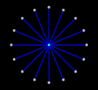
which uses a set of point-to-point muscles to drive the position of a single particle. The model consists of a single dynamic particle, initially located at the origin, attached to a set of 16 point-to-point muscles arranged radially around it. A tracking controller is created to control the excitations of these muscles so as to enable the particle to follow a trajectory specified by a probe. The code for the model, without the package and include directives, is listed below:

⬇

1 public class InverseParticle extends RootModel {

3 int numMuscles = 16; // num radial muscles surrounding the dynamic particle

4 double muscleStiffness = 200; // passive muscle stiffness

5 double muscleDamping = 1.0; // passive muscle damping

6 double muscleFmax = 1000; // max active force at excitation = 1

7 double dist = 1.0; // distance of anchor point from world origin

9 /**

10 * Create a muscle excitable spring extending out from the origin

11 * {@code part} at an angle {@code ang}.

12 */

13 void createMuscle (MechModel mech, Particle part, double ang) {

14 // create and add non-dynamic particle as fixed end point for muscle

15 Particle fixed = new Particle(

16 /*mass=*/1d, new Point3d(dist*Math.sin(ang),0.0,dist*Math.cos(ang)));

17 fixed.setDynamic(false);

18 mech.addParticle(fixed);

19 // create muscle and set its material

20 Muscle muscle = new Muscle (fixed, part);

21 muscle.setName ( // name the muscle using its angle

22 "muscle_"+Integer.toString((int)Math.round(Math.toDegrees(ang))));

23 muscle.setMaterial (

24 new SimpleAxialMuscle (muscleStiffness, muscleDamping, muscleFmax));

25 mech.addAxialSpring (muscle);

27 // make muscles red when activated

28 muscle.setExcitationColor (Color.RED);

29 muscle.setMaxColoredExcitation (0.5);

30 muscle.setRestLength (muscle.getLength());

31 }

33 public void build (String[] args) {

34 // create MechModel and add to RootModel

35 MechModel mech = new MechModel ("mech");

36 addModel (mech);

37 mech.setGravity (Vector3d.ZERO); // disable gravity

39 // create and add particle whose position is to be controlled

40 Particle part = new Particle ("center", /*mass=*/0.1, /*x,y,z=*/0, 0, 0);

41 part.setPointDamping (0.1); // add damping

42 mech.addParticle(part);

44 // create radial muscles connected to center particle

45 for (int i = 0; i < numMuscles; i++) {

46 double angle = 2*Math.PI*((double)i/numMuscles);

47 createMuscle (mech, part, angle);

48 }

50 // create the tracking controller and add it to the root model

51 TrackingController tcon = new TrackingController(mech, "tcon");

52 addController(tcon);

53 // set all muscles to be "exciters" for the controller to control

54 for (AxialSpring s : mech.axialSprings()) {

55 if (s instanceof Muscle) {

56 tcon.addExciter((Muscle)s);

57 }

58 }

59 // set the center dynamic particle to be the component that is tracked

60 TargetPoint target = tcon.addPointTarget(part);

61 // add an L-2 regularization term, since there are more muscles than

62 // target degrees-of-freedom

63 tcon.setL2Regularization(/*weight=*/0.1);

65 // Render properties: make points gray spheres, central particle white,

66 // and muscles as blue cylinders.

67 RenderProps.setSphericalPoints (this, dist/25, Color.LIGHT_GRAY);

68 RenderProps.setPointColor (part, Color.WHITE);

69 RenderProps.setCylindricalLines (mech, dist/50, Color.BLUE.darker ());

71 // add an input probe to control the position of the target:

72 NumericInputProbe targetprobe = new NumericInputProbe (

73 target, "position", /*startTime=*/0, /*stopTime=*/1);

74 targetprobe.setName ("target positions");

75 targetprobe.addData (

76 new double[] {0d,0d,0d, 0.5,0d,0.5, 0d,0d,0d}, // three knot points

77 /*timestep=*/0.5);

78 targetprobe.setInterpolationOrder (Interpolation.Order.Cubic);

79 addInputProbe (targetprobe);

81 // add an output probe to record the excitations:

82 NumericOutputProbe exprobe = InverseManager.createOutputProbe (

83 tcon, ProbeID.COMPUTED_EXCITATIONS, /*fileName=*/null,

84 /*startTime=*/0, /*stopTime=*/1, /*interval=*/-1);

85 addOutputProbe (exprobe);

86 }

87 }

The build() method begins by creating a MechModel in the usual way and disabling gravity (lines 35-37). The particle to be controlled is then created and placed at the origin and with a damping factor of 0.1 (lines 40-42). Next, the particle is attached to a set of point-to-point muscles that are arranged radially around it (lines 45-48). These are created using the method createMuscle() (lines 13-31), which attaches each to a fixed non-dynamic particle located a distance of dist from the origin, and sets its material to a SimpleAxialMuscle (Section 4.5.1.1) with a passive stiffness, damping and maximum force (at excitation 1) defined by muscleStiffness, muscleDamping, and muscleFmax (lines 4-6). Each muscle’s excitationColor and maxColoredExcitation property is set so that its color transitions to red as its excitation value varies from to (lines 28-29, Section 10.2.1.1)), and its rest length is initialized to its current length (line 30).

After the model components have been built, a TrackingController is created and added to the root model’s controller set (lines 51-52). All of the muscles are then added to the controller as exciters to be controlled (lines 54-58). The particle is added to the controller as a motion source using the addPointTarget() method (line 60), which returns a target object in the form of a TargetPoint. Since the number of exciters exceeds the degrees-of-freedom of the target space, an L2-regularization term is added (line 63) to resolve the redundancy.

Rendering properties are set at lines 67-69: points in the model are rendered as gray spheres, except for the dynamic particle which is colored white, and the muscles are drawn as blue cylinders. (The target particle, which is contained within the controller, is displayed using its default color of cyan.)

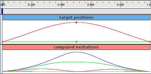
Probes are created to specify the target trajectory and record the computed excitations. The first, targetprobe, is an input probe attached to the position property of the target component, running from time 0 to 1 (lines 72-79). Its data is specified in code using addData(), which specifies three knot points with a time step of 0.5. Interpolation is set to cubic (line 78) for greater smoothness. The second, exprobe, is a probe that records all the excitations computed by the controller (lines 82-85). It is created by the utility method createOutputProbe() supplied by the InverseManager class (Section 10.4.1).

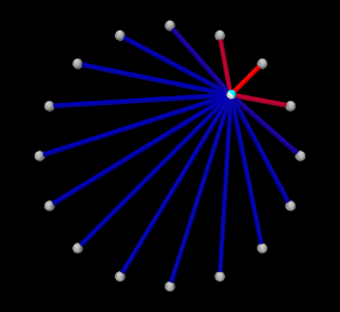
To run this example, select All demos > tutorial > InverseParticle from the Models menu. The model should load and initially appear as in Figure 10.3 (left). When run, the controller computes excitations to move the particle along the trajectory specified by the probe, which is upward and to the right (Figure 10.3, right) and back again.

The target point created by the controller is rendered separately from the source point as a cyan-colored sphere (see Section 10.2.2.2). As the simulation proceeds and certain muscles are excited, their coloring changes from blue to red, in proportion to their excitation, in accordance with the properties excitationColor and maxColoredExcitation. Recorded data for both the trajectory and the computed excitation probes are shown in Figure 10.4.

10 Inverse Simulation Bibliography 10.2 Tracking controller components

Generated on Wed Jul 24 21:23:12 2024 by LaTeXML [LOGO]