4.5 Point-to-point muscles, tendons and ligaments
Point-to-point muscles are a simple type of component in biomechanical models that provide muscle-activated forces acting along a line between two points. ArtiSynth provides this through Muscle, which is a subclass of AxialSpring that generates an active muscle force in response to its excitation property. The excitation property can be set and queried using the methods
As with AxialSprings, Muscle components use subclasses of
AxialMaterial to compute the
applied force ![]() in response to the muscle’s length
in response to the muscle’s length
![]() , length velocity
, length velocity ![]() , and excitation signal
, and excitation signal ![]() , which is
assumed to lie in the interval
, which is
assumed to lie in the interval ![]() . Special muscle
subclasses of AxialMaterial exist that compute forces that vary
in response to the excitation. As with other axial materials, this is
done by the material’s computeF() method, first described in
Section 3.1.7:
. Special muscle
subclasses of AxialMaterial exist that compute forces that vary
in response to the excitation. As with other axial materials, this is
done by the material’s computeF() method, first described in
Section 3.1.7:
Usually the force is the sum of a passive component plus an active component that arises in response to the excitation signal.
Once a muscle material is created, it can be assigned to a muscle or queried using Muscle methods
Muscle materials can also be assigned to axial springs, although the resulting force will always be computed with 0 excitation.
4.5.1 Simple muscle materials
A number of simple muscle materials are described below. All compute
force as a function of ![]() and
and ![]() , with an optional damping force
that is proportional to
, with an optional damping force
that is proportional to ![]() . More complex Hill-type muscles, with
force velocity curves, pennation angle, and a tendon component in
series, are also available and described in
Section 4.5.3.
. More complex Hill-type muscles, with
force velocity curves, pennation angle, and a tendon component in
series, are also available and described in
Section 4.5.3.
For historical reasons, the materials ConstantAxialMuscle, LinearAxialMuscle and PeckAxialMuscle, described below, contain a property called forceScaling that uniformly scales the computed force. This property is now deprecated, and should therefore have a value of 1. However, creating these materials with constructors not indicated in the documentation below will cause forceScaling to be set to a default value of 1000, thus requiring that the maximum force and damping values be correspondingly reduced.
4.5.1.1 SimpleAxialMuscle
SimpleAxialMuscle is the default AxialMaterial for Muscle, and is essentially an activated version of LinearAxialMaterial. It computes a simple force according to
| (4.1) |
where ![]() is the muscle rest length,
is the muscle rest length, ![]() and
and ![]() are stiffness and
damping terms, and
are stiffness and
damping terms, and ![]() is the maximum excitation force.
is the maximum excitation force. ![]() is
specified by the restLength property of the muscle component,
is
specified by the restLength property of the muscle component,
![]() by the excitation property of the Muscle, and
by the excitation property of the Muscle, and ![]() ,
, ![]() and
and ![]() by the following properties of SimpleAxialMuscle:
by the following properties of SimpleAxialMuscle:
| Property | Description | Default | |
|---|---|---|---|
| stiffness | stiffness term | 0 | |
| damping | damping term | 0 | |
| maxForce | maximum activation force that can be
imparted by |
1 |
SimpleAxialMuscles can be created with the following constructors:
where stiffness, damping, and fmax specify ![]() ,
, ![]() and
and ![]() , and properties are otherwise set to their defaults.
, and properties are otherwise set to their defaults.
4.5.1.2 ConstantAxialMuscle
ConstantAxialMuscle is a simple muscle material that has a contractile force proportional to its activation, a constant passive tension, and linear damping. The resulting force is described by:
| (4.2) |
The parameters ![]() ,
, ![]() and
and ![]() are specified as properties of
ConstantAxialMuscle:
are specified as properties of
ConstantAxialMuscle:
| Property | Description | Default | |
|---|---|---|---|
| maxForce | maximum contractile force | 1 | |
| passiveFraction | proportion of |
0 | |
| damping | damping parameter | 0 |
ConstantAxialMuscles can be created with the following factory methods and constructors:
where fmax, pfrac, and damping specify ![]() ,
, ![]() and
and ![]() , and properties are otherwise set to their defaults.
, and properties are otherwise set to their defaults.
Creating a ConstantAxialMuscle with the no-args constructor, or another constructor not listed above, will cause its forceScaling property (Section 4.5.1) to be set to 1000 instead of 1, thus requiring that fmax and damping be correspondingly reduced.
4.5.1.3 LinearAxialMuscle
LinearAxialMuscle is a simple muscle material that has a linear relationship between length and tension, as well as linear damping. Given a normalized length described by
| (4.3) |
the force generated by this material is:
| (4.4) |
The parameters are specified as properties of LinearAxialMaterial:
| Property | Description | Default | |
|---|---|---|---|
| maxForce | maximum contractile force | 1 | |
| passiveFraction | proportion of |
0 | |
| maxLength | length beyond which maximum passive and active forces are generated | 1 | |
| optLength | length below which zero active force is generated | 0 | |
| damping | damping parameter | 0 |
LinearAxialMuscles can be created with the following factory methods and constructors:
where fmax, lopt, lmax, pfrac and damping specify ![]() ,
, ![]() ,
, ![]() ,
, ![]() and
and ![]() ,
lrest specifies
,
lrest specifies ![]() and
and ![]() via
via
![]() and
and
![]() , and other properties are set to
their defaults.
, and other properties are set to
their defaults.
Creating a LinearAxialMuscle with the no-args constructor, or another constructor not listed above, will cause its forceScaling property (Section 4.5.1) to be set to 1000 instead of 1, thus requiring that fmax and damping be correspondingly reduced.
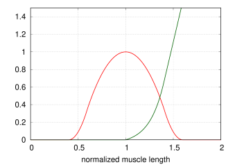
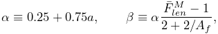
4.5.1.4 PeckAxialMuscle
The PeckAxialMuscle material generates a force as described in [19]. It has a typical Hill-type active force-length relationship (modeled as a cosine), but the passive force-length properties are linear. This muscle model was empirically verified for jaw muscles during wide jaw opening.
 |
 |
Given a normalized fibre length described by
| (4.5) |
and a normalized muscle length
| (4.6) |
the force generated by this material is:
 |
(4.7) |
The parameters are specified as properties of PeckAxialMuscle:
| Property | Description | Default | |
|---|---|---|---|
| maxForce | maximum contractile force | 1 | |
| passiveFraction | proportion of |
0 | |
| tendonRatio | tendon to fibre length ratio | 0 | |
| maxLength | length at which maximum passive force is generated | 1 | |
| optLength | length at which maximum active force is generated | 0 | |
| damping | damping parameter | 0 |
Figure 4.5 illustrates the force length relationship for a PeckAxialMuscle.
PeckAxialMuscles can be created with the following factory methods:
where fmax, lopt, lmax, tratio, pfrac
and damping specify ![]() ,
, ![]() ,
, ![]() ,
, ![]() ,
,
![]() and
and ![]() , and other properties are set to their defaults.
, and other properties are set to their defaults.
Creating a PeckAxialMuscle with the no-args constructor, or another constructor not listed above, will cause its forceScaling property (Section 4.5.1) to be set to 1000 instead of 1, thus requiring that fmax and damping be correspondingly reduced.
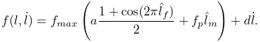
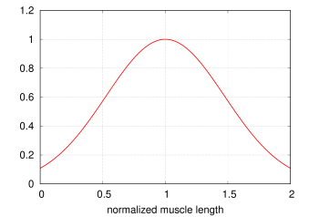
4.5.1.5 BlemkerAxialMuscle
The BlemkerAxialMuscle material generates a force as described in [5]. It is the axial muscle equivalent to the constitutive equation along the muscle fiber direction specified in the BlemkerMuscle FEM material.
 |
 |
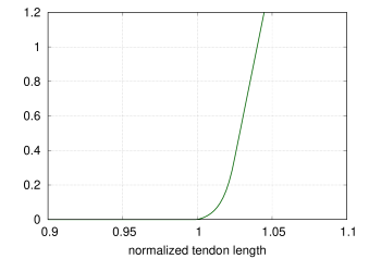
The force produced is a combination of active and passive terms, plus a damping term, given by
| (4.8) |
where ![]() is the maximum force,
is the maximum force, ![]() is the
normalized muscle length, and
is the
normalized muscle length, and
![]() and
and ![]() are the active and passive
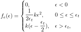
force length curves, given by
are the active and passive
force length curves, given by
![f_{L}(\hat{l})=\begin{cases}9\,(\hat{l}-0.4),&\hat{l}\in[0.4,0.6]\\
1-4(1-\hat{l}),&\hat{l}\in[0.6,1.4]\\
9\,(\hat{l}-1.6),&\hat{l}\in[1.4,1.6]\\
0,&\mathrm{otherwise},\\
\end{cases}](mi/mi1889.png) |
(4.9) |
and
![f_{P}(\hat{l})=\begin{cases}0,&\hat{l}<1\\
P_{1}(e^{P_{2}(\hat{l}-1)}-1),&\hat{l}\in[l_{opt},l_{max}/l_{opt}]\\
P_{3}\hat{l}+P_{4},&\hat{l}>l_{max}/l_{opt}.\\
\end{cases}](mi/mi1891.png) |
(4.10) |
For the passive force length curve, ![]() and
and ![]() are computed to
provide linear extrapolation for
are computed to
provide linear extrapolation for ![]() . The other
parameters are specified by properties of BlemkerAxialMuscle:
. The other
parameters are specified by properties of BlemkerAxialMuscle:
| Property | Description | Default | |
|---|---|---|---|
| maxForce | the maximum contractile force | ||
| expStressCoeff | exponential stress coefficient | 0.05 | |
| uncrimpingFactor | fibre uncrimping factor | 6.6 | |
| maxLength | length at which passive force becomes linear | 1.4 | |
| optLength | length at which maximum active force is generated | 1 | |
| damping | damping parameter | 0 |
Figure 4.6 illustrates the force length relationship for a BlemkerAxialMuscle.
BlemkerAxialMuscles can be created with the following constructors,
where lmax, lopt, fmax, ecoef, and uncrimp specify ![]() ,
, ![]() ,
, ![]() ,
, ![]() ,
, ![]() and
and
![]() , and properties are otherwise set to their defaults.
, and properties are otherwise set to their defaults.
4.5.2 Example: muscle attached to a rigid body
A simple model showing a single muscle connected to a rigid body is defined in
artisynth.demos.tutorial.SimpleMuscle
This model is identical to RigidBodySpring described in Section 3.2.2, except that the code to create the spring is replaced with code to create a muscle with a SimpleAxialMuscle material:
Also, so that the muscle renders differently, the rendering style for lines is set to SPINDLE using the convenience method
To run this example in ArtiSynth, select All demos > tutorial > SimpleMuscle from the Models menu. The model should load and initially appear as in Figure 4.7. Running the model (Section 1.5.3) will cause the box to fall and sway under gravity. To see the effect of the excitation property, select the muscle in the viewer and then choose Edit properties ... from the right-click context menu. This will open an editing panel that allows the muscle’s properties to be adjusted interactively. Adjusting the excitation property using the adjacent slider will cause the muscle force to vary.
4.5.3 Equilibrium muscles
ArtiSynth supplies several muscle materials that simulate a pennated
muscle in series with a tendon. Both the muscle and tendon generate
forces which are functions of their respective lengths ![]() and
and
![]() , and because these components are in series, their respective
forces must be equal when the system is in equilibrium. Given an
overall muscle-tendon length
, and because these components are in series, their respective
forces must be equal when the system is in equilibrium. Given an
overall muscle-tendon length ![]() , ArtiSynth solves
for
, ArtiSynth solves
for ![]() at each time step to ensure that this equilibrium condition
is met.
at each time step to ensure that this equilibrium condition
is met.

A general muscle-tendon system is illustrated by Figure
4.8, where ![]() and
and ![]() are the muscle and
tendon lengths. These two components generate forces given by
are the muscle and
tendon lengths. These two components generate forces given by
![]() and
and ![]() , where
, where ![]() , and the
fact that these components are in series implies that their forces
must be in equilibrium:
, and the
fact that these components are in series implies that their forces
must be in equilibrium:
| (4.11) |
The muscle force is in turn produced by a fibre force ![]() acting at a pennation angle
acting at a pennation angle ![]() with respect to the
principal muscle direction, such that
with respect to the
principal muscle direction, such that
where ![]() is the fibre length, which satisfies
is the fibre length, which satisfies
![]() , and
, and ![]() .
.
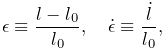
The fibre force is usually computed from the normalized fibre length
![]() and normalized fibre velocity
and normalized fibre velocity ![]() , defined by
, defined by
| (4.12) |
where ![]() is the optimal fibre length and
is the optimal fibre length and ![]() is the maximum
contraction velocity. It is composed of three components in parallel,
such that
is the maximum
contraction velocity. It is composed of three components in parallel,
such that
| (4.13) |
where ![]() is the maximum isometric force,
is the maximum isometric force,
![]() is the active force term induced by an
activation level
is the active force term induced by an
activation level ![]() and modulated by the active force length
curve
and modulated by the active force length
curve ![]() and the force velocity curve
and the force velocity curve ![]() ,
,
![]() is the passive force length curve, and
is the passive force length curve, and ![]() is an optional damping term induced by a fibre damping parameter
is an optional damping term induced by a fibre damping parameter
![]() .
.
The tendon force ![]() is computed from
is computed from
where ![]() is (again) the maximum isometric force,
is (again) the maximum isometric force, ![]() is the
tendon force length curve and
is the
tendon force length curve and ![]() is the normalized tendon
length, defined by dividing
is the normalized tendon
length, defined by dividing ![]() by the tendon slack length
by the tendon slack length
![]() :
:
As the muscle moves, it is assumed that the height ![]() from the fibre
origin to the main muscle line of action remains constant.
This height is defined by
from the fibre
origin to the main muscle line of action remains constant.
This height is defined by
where ![]() is the optimal pennation angle at the optimal
fibre length when
is the optimal pennation angle at the optimal
fibre length when ![]() .
.
4.5.4 Equilibrium muscle materials
The equilibrium muscle materials supplied by ArtiSynth include Thelen2003AxialMuscle and Millard2012AxialMuscle. These are all controlled by properties which specify the parameters presented in Section 4.5.3:
| Property | Description | Default | |
|---|---|---|---|
| maxIsoForce | maximum isometric force | 1000 | |
| optFibreLength | optimal fibre length | 0.1 | |
| tendonSlackLength | length beyond which tendon exerts force | 0.2 | |
| optPennationAngle | pennation angle at optimal fibre length (radians) | 0 | |
| maxContractionVelocity | maximum contraction velocity | 10 | |
| fibreDamping | damping parameter for normalized fibre velocity | 0 |
The materials differ from each other with respect to their active,
passive and tendon force length curves (![]() ,
, ![]() , and
, and
![]() ) and their force velocity curves (
) and their force velocity curves (![]() ).
).
For a given muscle instance, it is typically only necessary to specify
![]() ,
, ![]() ,
, ![]() and
and ![]() , where
, where ![]() ,
, ![]() and
and ![]() are given
in the model’s basic force and length units.
are given
in the model’s basic force and length units. ![]() is given in units
of
is given in units
of ![]() per second and has a default value of 10; changing this value
will stretch or contract the domain of the force velocity curve
per second and has a default value of 10; changing this value
will stretch or contract the domain of the force velocity curve
![]() . The damping parameter
. The damping parameter ![]() imparts a damping force
proportional to
imparts a damping force
proportional to ![]() and has a default value of 0 (i.e., no
damping). It is often not necessary to add fibre damping (since
damping can be readily applied to the model in other ways), but
and has a default value of 0 (i.e., no
damping). It is often not necessary to add fibre damping (since
damping can be readily applied to the model in other ways), but
![]() is supplied for formulations that do specify damping. If
non-zero,
is supplied for formulations that do specify damping. If
non-zero, ![]() is usually set to a value less than or equal to
is usually set to a value less than or equal to
![]() .
.
In addition to the above parameters, equilibrium muscle materials also export the following properties to adjust their behavior:
| Property | Description | Default |
|---|---|---|
| rigidTendon | forces the tendon to be rigid | false |
| ignoreForceVelocity | ignore the force velocity curve |
false |
If rigidTendon is true, the tendon will be assumed to be
rigid with a length given by the tendon slack length parameter ![]() .
This simplifies the muscle computations since
.
This simplifies the muscle computations since ![]() is then given by
is then given by
![]() and there is no need to compute an equilibrium position.
If ignoreForceVelocity is true, then force velocity
effects are ignored by replacing the force velocity curve
and there is no need to compute an equilibrium position.
If ignoreForceVelocity is true, then force velocity
effects are ignored by replacing the force velocity curve ![]() with
with ![]() .
.
The different equilibrium muscle materials are now summarized:
4.5.4.1 Millard2012AxialMuscle
Millard2012AxialMuscle implements the default version of the Millard2012EquilibriumMuscle model supplied by OpenSim [7] and described in [15].
The active, passive and tendon force length curves (![]() ,
,
![]() , and
, and ![]() ) and force velocity curve (
) and force velocity curve (![]() )
are implemented using cubic Hermite spline curves to conform closely
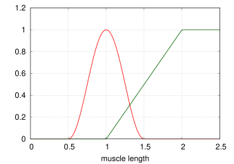
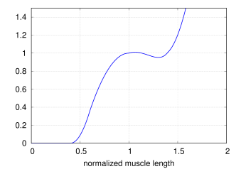
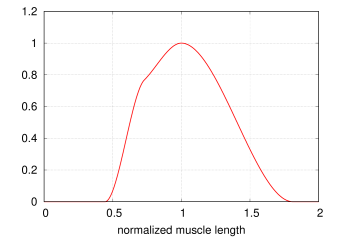
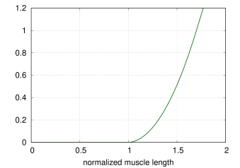
to the default curve values provided by OpenSim’s Millard2012EquilibriumMuscle. Plots of these curves are shown in
Figures 4.9 and 4.10. Both
the passive and tendon force curves are linearly extrapolated (and
hence exhibit constant stiffness) past
)
are implemented using cubic Hermite spline curves to conform closely
to the default curve values provided by OpenSim’s Millard2012EquilibriumMuscle. Plots of these curves are shown in
Figures 4.9 and 4.10. Both
the passive and tendon force curves are linearly extrapolated (and
hence exhibit constant stiffness) past ![]() and
and
![]() , respectively, with stiffness values of 2.857 and
29.06.
, respectively, with stiffness values of 2.857 and
29.06.
 |
 |
 |
 |
OpenSim requires that the Millard2012EquilibriumMuscle always exhibits a small bias activation, even when the activation should be zero, in order to avoid a singularity in the computation of the muscle length. ArtiSynth computes the muscle length in a manner that makes this unnecessary.
Millard2012AxialMuscles can be created using the constructors
where fmax, lopt, tslack, and optPenAng
specify ![]() ,
, ![]() ,
, ![]() , and
, and ![]() , and other properties are
set to their defaults.
, and other properties are
set to their defaults.
4.5.4.2 Thelen2003AxialMuscle
Thelen2003AxialMuscle implements the Thelen2003Muscle model supplied by OpenSim [7] and introduced in [27].
The active and passive force length curves are described by
| (4.14) |
and
| (4.15) |
where ![]() ,
, ![]() , and
, and ![]() are parameters, described
in [27], that control the curve shapes. These
are exposed as properties of Thelen2003AxialMuscle and are
described in Table 4.3.
are parameters, described
in [27], that control the curve shapes. These
are exposed as properties of Thelen2003AxialMuscle and are
described in Table 4.3.
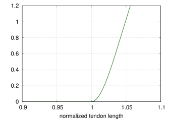
The tendon force length curve is described by
 |
(4.16) |
where ![]() ,
, ![]() ,
, ![]() and
and ![]() are
parameters, described in [27], that control the
curve shape. The values of these are either fixed, or derived from the
maximum isometric tendon strain
are
parameters, described in [27], that control the
curve shape. The values of these are either fixed, or derived from the
maximum isometric tendon strain ![]() (controlled by the
fmaxTendonStrain property, Table 4.3),
according to
(controlled by the
fmaxTendonStrain property, Table 4.3),
according to
 |
(4.17) |
| Property | Description | Default | |
|---|---|---|---|
| kShapeActive | shape factor for active force length curve | 0.45 | |
| kShapePassive | shape factor for active force length curve | 5.0 | |
| fmaxMuscleStrain | passive muscle strain at maximum isometric muscle force | 0.6 | |
| fmaxTendonStrain | tendon strain at maximum isometric muscle force | 0.04 | |
| af | force velocity shape factor | 0.25 | |
| flen | maximum normalized lengthening force | 1.4 | |
| fvLinearExtrapThreshold |
|
0.95 |
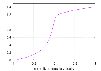
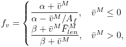
The force velocity curve is determined from equation (6)
in [27]. In the notation used by that equation
and the accompanying equation (7), ![]() ,
, ![]() , and
, and ![]() . Inverting equation
(6) yields the force velocity curve:
. Inverting equation
(6) yields the force velocity curve:
 |
where
 |
and ![]() is the activation level. Parameters include the maximum
normalized lengthening force
is the activation level. Parameters include the maximum
normalized lengthening force ![]() , and force velocity shape factor
, and force velocity shape factor
![]() , described in Table 4.3.
, described in Table 4.3.
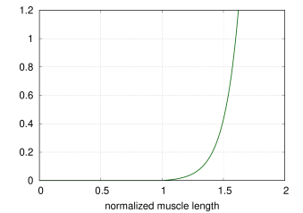
Plots of the curves resulting from the above equations are shown, for default values, in Figures 4.11 and 4.12.
 |
 |
 |
 |
Thelen2003AxialMuscles can be created using the constructors
where fmax, lopt, tslack, and optPenAng
specify ![]() ,
, ![]() ,
, ![]() , and
, and ![]() , and other properties are
set to their defaults.
, and other properties are
set to their defaults.
4.5.5 Tendons and ligaments
Special point-to-point spring materials are also available to model tendons and ligaments. Because these are passive materials, they would normally be assigned to AxialSpring instead of Muscle components, although they will also work correctly in the latter. The materials include:
4.5.5.1 Millard2012AxialTendon
Millard2012AxialTendon implements the default tendon material of the Millard2012AxialMuscle (Section 4.5.4.1), with a force length relationship given by
| (4.18) |
where ![]() is the maximum isometric force,
is the maximum isometric force, ![]() is the tendon
force length curve (shown in Figure 4.10,
right), and
is the tendon
force length curve (shown in Figure 4.10,
right), and ![]() is the tendon slack length.
is the tendon slack length. ![]() and
and ![]() are specified
by the following properties of Millard2012AxialTendon:
are specified
by the following properties of Millard2012AxialTendon:
| Property | Description | Default | |
|---|---|---|---|
| maxIsoForce | maximum isometric force | 1000 | |
| tendonSlackLength | length beyond which tendon exerts force | 0.2 |
Millard2012AxialTendons can be created with the constructors
where fmax and tslack specify ![]() and
and ![]() , and
other properties are set to their defaults.
, and
other properties are set to their defaults.
4.5.5.2 Thelen2003AxialTendon
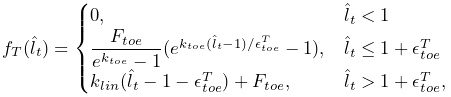
Thelen2003AxialTendon implements the default tendon material of the Thelen2003AxialMuscle (Section 4.5.4.2), with a force length relationship given by
| (4.19) |
where ![]() is the maximum isometric force,
is the maximum isometric force, ![]() is the tendon
force length curve described by equation (4.16),
and
is the tendon
force length curve described by equation (4.16),
and ![]() is the tendon slack length.
is the tendon slack length. ![]() ,
, ![]() , and the maximum
isometric tendon strain
, and the maximum
isometric tendon strain ![]() (used to determine the parameters
of (4.16), according to (4.17)),
are specified by the following properties of Thelen2003AxialTendon:
(used to determine the parameters
of (4.16), according to (4.17)),
are specified by the following properties of Thelen2003AxialTendon:
| Property | Description | Default | |
|---|---|---|---|
| maxIsoForce | maximum isometric force | 1000 | |
| tendonSlackLength | length beyond which tendon exerts force | 0.2 | |
| fmaxTendonStrain | tendon strain at maximum isometric muscle force | 0.04 |
Thelen2003AxialTendons can be created with the constructors
where fmax and tslack specify ![]() and
and ![]() , and
other properties are set to their defaults.
, and
other properties are set to their defaults.
4.5.5.3 Blankevoort1991AxialLigament
Blankevoort1991AxialLigament implements the Blankevoort1991Ligament model supplied by OpenSim [7] and described in [4, 24].
With the ligament strain and its derivative defined by
 |
(4.20) |
the ligament force is given by
| (4.21) |
where
 |
and
 |
The parameters ![]() ,
, ![]() ,
, ![]() , and
, and ![]() are specified by the following
properties of Blankevoort1991Ligament:
are specified by the following
properties of Blankevoort1991Ligament:
| Property | Description | Default | |
|---|---|---|---|
| slackLength | ligament slack length | 0 | |
| transitionStrain | strain at transition from toe to linear | 0.06 | |
| linearStiffness | maximum stiffness of force-length curve | 100 | |
| damping | damping parameter | 0.003 |
Blankevoort1991Ligaments can be created with the constructors
where stiffness, slackLen and damping specify ![]() ,
,
![]() and
and ![]() , and other properties are set to their defaults.
, and other properties are set to their defaults.
4.5.6 Example: muscles with separate tendons
An alternate way to model the equilibrium muscles of Section
4.5.3 is to use two separate
point-to-point muscles, attached in series via a connecting particle
with a small mass (and possibly damping), thus implementing the muscle
and tendon components separately. This approach allows the muscle
equilibrium length to be determined automatically by the physical
response of the connecting particle, in a manner similar to that
employed by OpenSim’s Millard2012AccelerationMuscle (described
in [14]). For the muscle material, one
can use any of the tendonless materials of Section
4.5.1, or the materials of Section
4.5.3 with the properties rigidTendon and
tendonSlackLength set to true and ![]() , respectively, while
the tendon material can be one described in Section
4.5.5 or some other suitable passive material.
The implicit integrators used by ArtiSynth should permit relatively
stable simulation of the arrangement.
, respectively, while
the tendon material can be one described in Section
4.5.5 or some other suitable passive material.
The implicit integrators used by ArtiSynth should permit relatively
stable simulation of the arrangement.
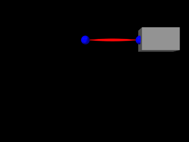
While it is usually easier to employ the equilibrium muscle materials of Section 4.5.4, especially for models involving wrapping and/or via points (Chapter 9) where it may be difficult to handle the connecting particle correctly, in some situations the separate muscle/tendon method may offer a more versatile solution. It can also be used to validate the equilibrium muscles, as illustrated by the application model defined in
artisynth.demos.tutorial.EquilibriumMuscleDemo
which provides a direct comparison of the methods. It creates two simple instances of a Millard 2012 muscle, one above the other in the x-z plane, with the top instance implemented using the separate muscle/tendon method and the bottom instance implemented using an equilibrium muscle material (Figure 4.13). The application model uses control and monitoring components introduced in Chapter 5 to drive the simulation and record its results: a controller (Section 5.3) is used to uniformly extend the length of both muscles; output probes (Section 5.4) are used to record the resulting tension forces; and a control panel (Section 5.1) is created to allow the user to interactively adjust some of the muscle parameters.
The code for the EquilibriumMuscleDemo class attributes and build() method is shown below:
Lines 4-10 declare attributes for muscle parameters and the initial length of the combined muscle-tendon. Within the build() method, a MechModel is created with zero gravity (lines 14-16).
Next, the separate muscle/tendon muscle is assembled, consisting of
three particles (pl0, pc0, and pr0, lines 20-30), a
muscle mus0 connected between pl0 and pc0 (lines
33-39), and a tendon connected between pc0 and pr0
(lines 42-45). Particles pl0 and pr0 are both set to be
non-dynamic, since pl0 will be fixed and pr0 will be moved
parametrically, while the connecting particle pc0 has a small
mass and its position is updated by the simulation and so
automatically maintains force equilibrium between the muscle and
tendon. The material mat0 used for mus0 is an instance of
Millard2012AxialMuscle, with the tendon removed by setting the
tendonSlackLength and rigidTendon properties to ![]() and
true, respectively, while the material for tendon is an
instance of Millard2012AxialTendon.
and
true, respectively, while the material for tendon is an
instance of Millard2012AxialTendon.
The equilibrium muscle is then assembled, consisting of two particles (pl1 and pr1, lines 49-55) and a muscle mus1 connected between them (lines 57-61). pl1 and pr1 are both set to be non-dynamic, since pl1 will be fixed and pr1 will be moved parametrically, and the material mat1 for mus1 is an instance of Millard2012AxialMuscle in its default equilibrium mode. Excitations for both mus0 and mus1 are initialized to 1, and the zero-velocity equilibrium muscle length is computed using mat1.computeLmWithConstantVm() (lines 65-69). This is used to update the muscle position, for mus0 by setting the x coordinate of pc0 and for mus1 by setting the internal muscle length variable of mat1 (lines 71-72).
Render properties for different components are set at lines 76-80, and then a control panel is created to allow interactive adjustment of the muscle material properties optPennationAngle, fibreDamping, and ignoreForceVelocity, as well the muscle excitations (lines 83-88). As explained in Sections 5.1.1 and 5.1.3, addWidget() methods are used to create widgets that control each of these properties for both mus0 and mus1.
At line 92, a controller is added to the root model to move the
right side particles p0r and p1r during the simulation,
thus changing the muscles’ lengths and hence their tension
forces. Controllers are explained in Section
5.3, and the controller itself is defined
by lines 101-127 of the code listing below. At the start of each
simulation time step, the controller’s apply() method is called,
with t0 and t1 denoting the step’s start and end times.
It increases the x positions of p0r and p1r uniformly with
a speed of mySpeed until time myRunTime/2, and then
reverses direction until time myRunTime. Velocities are also
updated since these are needed to determine ![]() for the muscles’
computeF() methods.
for the muscles’
computeF() methods.
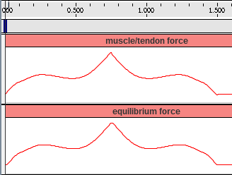
Each muscle’s tension force is recorded by an output probe connected to its forceNorm property. Probes are explained in Section 5.4; in this example, they are created using the convenience method addForceProbe(), defined by lines 130-140 (below) and called at lines 93-94 in the build() method, with probes for the muscle/tendon and equilibrium muscles named “muscle/tendon force” and “equilibrium force”, respectively.
 |
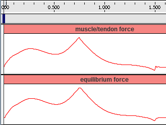 |
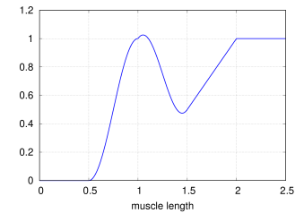
To run this example in ArtiSynth, select All demos > tutorial > EquilibriumMuscleDemo from the Models menu. The model should load and initially appear as in Figure 4.13. As explained above, running the model will cause the muscles to be extended and contracted by moving particles p0r and p1r right and back again. As this happens, the resulting tension forces can be examined by expanding the output probes in the timeline (see section “The Timeline” in the ArtiSynth User Interface Guide). The results are shown in Figure 4.14, with the left and right images showing results with the muscle material property ignoreForceVelocity set to true and false, respectively.
As should be expected, the results for the two muscle implementations are very similar. In both cases, the forces exhibit a local peak near time 0.25 when the muscle lengths are at the maximum of the active force length curve. As time increases, forces then decrease and then rise again as the passive force increases, peaking at time 0.75 when the muscle starts to contract. In the left image, the forces during contraction are symmetrical with those during extension, while in the right image the post-peak forces are more attenuated, because in the latter case the force velocity relationship is enabled as this reduces forces when a muscle is contracting.
![[LOGO]](data:image/png;base64,iVBORw0KGgoAAAANSUhEUgAAAAsAAAAOCAYAAAD5YeaVAAAAAXNSR0IArs4c6QAAAAZiS0dEAP8A/wD/oL2nkwAAAAlwSFlzAAALEwAACxMBAJqcGAAAAAd0SU1FB9wKExQZLWTEaOUAAAAddEVYdENvbW1lbnQAQ3JlYXRlZCB3aXRoIFRoZSBHSU1Q72QlbgAAAdpJREFUKM9tkL+L2nAARz9fPZNCKFapUn8kyI0e4iRHSR1Kb8ng0lJw6FYHFwv2LwhOpcWxTjeUunYqOmqd6hEoRDhtDWdA8ApRYsSUCDHNt5ul13vz4w0vWCgUnnEc975arX6ORqN3VqtVZbfbTQC4uEHANM3jSqXymFI6yWazP2KxWAXAL9zCUa1Wy2tXVxheKA9YNoR8Pt+aTqe4FVVVvz05O6MBhqUIBGk8Hn8HAOVy+T+XLJfLS4ZhTiRJgqIoVBRFIoric47jPnmeB1mW/9rr9ZpSSn3Lsmir1fJZlqWlUonKsvwWwD8ymc/nXwVBeLjf7xEKhdBut9Hr9WgmkyGEkJwsy5eHG5vN5g0AKIoCAEgkEkin0wQAfN9/cXPdheu6P33fBwB4ngcAcByHJpPJl+fn54mD3Gg0NrquXxeLRQAAwzAYj8cwTZPwPH9/sVg8PXweDAauqqr2cDjEer1GJBLBZDJBs9mE4zjwfZ85lAGg2+06hmGgXq+j3+/DsixYlgVN03a9Xu8jgCNCyIegIAgx13Vfd7vdu+FweG8YRkjXdWy329+dTgeSJD3ieZ7RNO0VAXAPwDEAO5VKndi2fWrb9jWl9Esul6PZbDY9Go1OZ7PZ9z/lyuD3OozU2wAAAABJRU5ErkJggg==)