5.4 Probes
In addition to controllers and monitors, applications can also attach streams of data, known as probes, to input and output values associated with the simulation. Probes derive from the same base class ModelAgentBase as controllers and monitors, but differ in that
-
1.
They are associated with an explicit time interval during which they are applied;
-
2.
They can have an attached file for supplying input data or recording output data;
-
3.
They are displayable in the ArtiSynth timeline panel.
A probe is applied (by calling its apply() method) only for time steps that fall within its time interval. This interval can be set and queried using the following methods:
The probe’s attached file can be set and queried using:
where filePath is a string giving the file’s path name. If filePath is relative (i.e., it does not start at the file system root), then it is assumed to be relative to the ArtiSynth working folder, which can be queried and set using the methods
of ArtisynthPath. The working folder can also be set from the ArtiSynth GUI by choosing File > Set working folder ....
If not explicitly set within the application, the working folder will default to a system dependent setting, which may be the user’s home folder, or the working folder of the process used to launch Artisynth.
Details about the timeline display can be found in the section “The Timeline” in the ArtiSynth User Interface Guide.
There are two types of probe: input probes, which are applied at the beginning of each simulation step before the controllers, and output probes, which are applied at the end of the step after the monitors. This is described in Section 1.2.1, and in even further detail in the “Advancing Models in Time” section of the ArtiSynth Reference Manual.
While applications are free to construct any type of probe by subclassing either InputProbe or OutputProbe, most applications utilize either NumericInputProbe or NumericOutputProbe, which explicitly implement streams of numeric data which are connected to properties of various model components. The remainder of this section will focus on numeric probes.
As with controllers and monitors, probes also implement a isActive() method that indicates whether or not the probe is active. Probes that are not active are not invoked. Probes also provide a setActive() method to control this setting, and export it as the property active. This allows probe activity to be controlled at run time.
To enable or disable a probe at run time, locate it in the navigation panel (under the RootModel’s inputProbes or outputProbes list), chose Edit properties ... from the right-click context menu, and set the active property as desired.
Probes can also be enabled or disabled in the timeline, by either selecting the probe and invoking activate or deactivate from the right-click context menu, or by clicking the track mute button (which activates or deactivates all probes on that track).
5.4.1 Numeric probe structure
Numeric probes are associated with:
-
•
A vector of temporally-interpolated numeric data;
-
•
One or more properties to which the probe is bound and which are either set by the numeric data (input probes), or used to set the numeric data (output probes).
The numeric data is implemented internally by a
NumericList, which stores the data
as a series of vector-valued knot points at prescribed times ![]() and
then interpolates the data for an arbitrary time
and
then interpolates the data for an arbitrary time ![]() using an
interpolation scheme provided by
Interpolation.
using an
interpolation scheme provided by
Interpolation.
Some of the numeric probe methods associated with the interpolated data include:
Interpolation schemes are described by the enumerated type Interpolation.Order and presently include:
- Step
-
Values at time
 are set to the values of the closest knot point
 such that
  .
. - Linear
-
Values at time
are set by linear interpolation of the knot points
 such that
 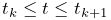 .
. - Parabolic
-
Values at time
are set by quadratic interpolation of the knots
 such that .
 - Cubic
-
Values at time
are set by cubic Catmull interpolation of the knots
 such that .
Each property bound to a numeric probe must have a value that can be mapped onto a scalar or vector value. Such properties are know as numeric properties, and whether or not a value is numeric can be tested usingNumericConverter.isNumeric(value).
By default, the total number of scalar and vector values associated with all the properties should equal the size of the interpolated vector (as returned by getVsize()). However, it is possible to establish more complex mappings between the property values and the interpolated vector. These mappings are beyond the scope of this document, but are discussed in the sections “General input probes” and “General output probes” of the ArtiSynth User Interface Guide.
5.4.2 Creating probes in code
This section discusses how to create numeric probes in code. They can also be created and added to a model graphically, as described in the section “Adding and Editing Numeric Probes” in the ArtiSynth User Interface Guide.
Numeric probes have a number of constructors and methods that make it relatively easy to create instances of them in code. For NumericInputProbe, there is the constructor
which creates a NumericInputProbe, binds it to a property located relative to the component c by propPath, and then attaches it to the file indicated by filePath and loads data from this file (see Section 5.4.4). The probe’s start and stop times are specified in the file, and its vector size is set to match the size of the scalar or vector value associated with the property.
To create a probe attached to multiple properties, one may use the constructor
which binds the probe to multiple properties specified relative to c by propPaths. The probe’s vector size is set to the sum of the sizes of the scalar or vector values associated with these properties.
For NumericOutputProbe, one may use the constructor
which creates a NumericOutputProbe, binds it to the property propPath located relative to c, and then attaches it to the file indicated by filePath. The argument interval indicates the update interval associated with the probe, in seconds; a value of 0.01 means that data will be added to the probe every 0.01 seconds. If interval is specified as -1, then the update interval will default to the simulation step size. This interval can also be accessed after the probe is created using
To create an output probe attached to multiple properties, one may use the constructor
As the simulation proceeds, an output probe will accumulate data, but this data will not be saved to any attached file until the probe’s save() method is called. This can be requested in the GUI for all probes by clicking on the Save button in the timeline toolbar, or for specific probes by selecting them in the navigation panel (or the timeline) and then choosing Save data in the right-click context menu.
Output probes created with the above constructors have a default interval of [0, 1]. A different interval may be set using setInterval(), setStartTime(), or setStopTime().
5.4.3 Example: probes connected to SimpleMuscle
A model showing a simple application of probes is defined in
artisynth.demos.tutorial.SimpleMuscleWithProbes
This extends SimpleMuscle (Section 4.5.2) to add an input probe to move particle p1 along a defined path, along with an output probe to record the velocity of the frame marker. The complete class definition is shown below:
The input and output probes are added using the custom methods createInputProbe() and createOutputProbe(). At line 14, createInputProbe() creates a new input probe bound to the targetPosition property for the component particles/p1 located relative to the MechModel mech. The same constructor attaches the probe to the filesimpleMuscleP1Pos.txt, which is read to load the probe data. The format of this and other probe data files is described in Section 5.4.4. The method PathFinder.getSourceRelativePath() is used to locate the file relative to the source directory for the application model (see Section 2.6). The probe is then given the name "Particle Position" (line 18) and added to the root model (line 19).
Similarly, createOutputProbe() creates a new output probe which is bound to the velocity property for the component frameMarkers/0 located relative to mech, is attached to the file simpleMuscleMkrVel.txt located in the application model source directory, and is assigned an update interval of 0.01 seconds. This probe is then named "FrameMarker Velocity" and added to the root model.
The build() method calls super.build() to create everything required for SimpleMuscle, calls createInputProbe() and createOutputProbe() to add the probes, and adjusts the MechModel viewer bounds to make the resulting probe motion more visible.
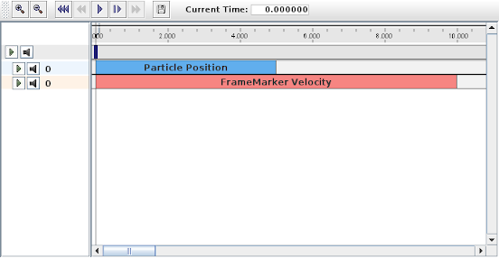
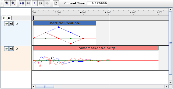
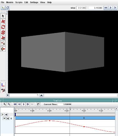
To run this example in ArtiSynth, select All demos > tutorial > SimpleMuscleWithProbes from the Models menu. After the model is loaded, the input and output probes should appear on the timeline (Figure 5.6). Expanding the probes should display their numeric contents, with the knot points for the input probe clearly visible. Running the model will cause particle p1 to trace the trajectory specified by the input probe, while the velocity of the marker is recorded in the output probe. Figure 5.7 shows an expanded view of both probes after the simulation has run for about six seconds.
5.4.4 Data file format
The data files associated with numeric probes are ASCII files containing two lines of header information followed by a set of knot points, one per line, defining the numeric data. The time value (relative to the probe’s start time) for each knot point can be specified explicitly at the start of the each line, in which case the file takes the following format:
Knot point information begins on line 3, with each line being a
sequence of numbers giving the knot’s time followed by ![]() values,
where
values,
where ![]() is the vector size of the probe (i.e., the value returned by
getVsize()).
is the vector size of the probe (i.e., the value returned by
getVsize()).
Alternatively, time values can be implicitly specified starting at 0 (relative to the probe’s start time) and incrementing by a uniform timeStep, in which case the file assumes a second format:
For both formats, startTime, startTime, and scale are numbers giving the probe’s start and stop time in seconds and scale gives the scale factor (which is typically 1.0). interpolation is a word describing how the data should be interpolated between knot points and is the string value of Interpolation.Order as described in Section 5.4.1 (and which is typically Linear, Parabolic, or Cubic). vsize is an integer giving the probe’s vector size.
The last entry on the second line is either a number specifying a (uniform) time step for the knot points, in which case the file assumes the second format, or the keyword explicit, in which case the file assumes the first format.
As an example, the file used to specify data for the input probe in the example of Section 5.4.3 looks like the following:
Since the data is uniformly spaced beginning at 0, it would also be possible to specify this using the second file format:
5.4.5 Adding input probe data in code
It is also possible to specify input probe data directly in code, instead of reading it from a file. For this, one would use the constructor
which creates a NumericInputProbe with the specified property and with start and stop times indicated by t0 and t1. Data can then be added to this probe using the method
where data is an array of knot point data. This contains the
same knot point information as provided by a file (Section
5.4.4), arranged in row-major order. Times values
for the knots are either implicitly specified, starting at 0 (relative
to the probe’s start time) and increasing uniformly by the amount
specified by timeStep, or are explicitly specified at the
beginning of each knot if timeStep is set to the built-in
constant NumericInputProbe.EXPLICIT_TIME. The size of the data array should then be either ![]() (implicit time values) or
(implicit time values) or
![]() (explicit time values), where
(explicit time values), where ![]() is the probe’s vector size
and
is the probe’s vector size
and ![]() is the number of knots.
is the number of knots.
As an example, the data for the input probe in Section 5.4.3 could have been specified using the following code:
When specifying data in code, the interpolation defaults to Linear unless explicitly specified usingsetInterpolationOrder(), as in, for example:
Data can also be added incrementally, using the method
which adds a data knot the specified values at time t; values should have a size equal to the probe’s vector size. For example, the array-based example above could instead by implemented as
When an input probe is created without data specified in its constructor (e.g., by means of a probe data file), then it automatically adds knot points at its start and end times, with values set from the current values of its bound properties. Applying such a probe, without adding additional data, will thus leave the values of its properties unchanged.
The addData() methods described above do not remove existing knot points (although they will overwrite knots that exist at the same times). In order to replace all data, one can first call the method
which removes all knot points. Probes with no knots assign 0 to all their property values. Data can subsequently be added using the addData() methods. Alternatively, one can call
which behaves identically to the addData(double[],timeStep) method except that it first removes all existing data.
5.4.5.1 Extending data to the start and end
By explicitly using the clearData() or setData() methods, it is possible to create an input probe for which data is missing at its start and/or stop times. The behavior in that case is determined by the probe’s extendData property: if the property is set to true, then data values between the start time and the first knot, or the last knot and the stop time, are set to the values of the first and last knot, respectively. Otherwise, these data values are set to zero.
As with all properties, extendData can be set and queried in code using the accessors
The default value of extendData is true. As mentioned above, probes with no data set their data values uniformly to 0.
5.4.6 Setting data from text or CSV files and other probes
Applications can import/export data from/to text and CSV files. For both
formats, the file is assumed to contain one line per time value, with numbers
separated by either whitespace (for text) or a comma character (for CSV). Time
values may or may not be included; if ![]() is the probe’s vector size, each line
will have
is the probe’s vector size, each line
will have ![]() values in the former case and
values in the former case and ![]() in the latter. As an
example, a text file including time values for a probe with
in the latter. As an
example, a text file including time values for a probe with ![]() and four
time values might look like
and four
time values might look like
while an equivalent CSV file could look like
Importing and exporting can be done by the following methods:
| void importTextData (File file, double timeStep) |
Import from a text file. |
| void exportTextData (File file) |
Export to a text file. |
| void exportTextData (File file, String fmtStr, boolean includeTime) |
Export to a text file. |
| void importCsvData (File file, double timeStep) |
Import from a CSV file. |
| void exportCsvData (File file) |
Export to a CSV file. |
| void exportCsvData (File file, String fmtStr, boolean includeTime) |
Export to a CSV file. |
| void importData (File file, double timeStep) |
Infer text or CSV from file suffix. |
The timeStep argument to the import methods indicates whether the file
includes time values: if it is ![]() , time values should be included;
otherwise, time values are computed from k*timeStep, where k is the
the line number starting at 0. The arguments fmtStr and includeTime
for some of the export methods specify a C-style numeric format string
(see NumberFormat) and whether or not time values
should be included; the defaults are "%g" (full general precision) and
true.
, time values should be included;
otherwise, time values are computed from k*timeStep, where k is the
the line number starting at 0. The arguments fmtStr and includeTime
for some of the export methods specify a C-style numeric format string
(see NumberFormat) and whether or not time values
should be included; the defaults are "%g" (full general precision) and
true.
It is also possible to copy data from one probe to another, using the method
| void setData (NumericProbeBase src, boolean useAbsoluteTime) |
All knot points and values are copied from src, which can be any numeric probe (input or output), with the only restriction being that its vector size must equal or exceed that of the calling probe (extra values are ignored). If useAbsoluteTime is true, time values are mapped between the probes using absolute time; otherwise, probe relative time is used. When using this method, care should be taken to ensure that the there will be knot points to cover the start and stop times of the calling probe.
5.4.7 Tracing probes
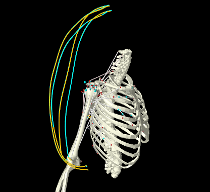
It is often useful to follow the path or evolution of a position or vector quantity as it evolves in time during a simulation. For example, one may wish to trace out the path of some points, as per Figure 5.8, which traces the actual and desired paths of some marker points during an inverse simulation of the type described in Chapter 10.
ArtiSynth supplies TracingProbes that can be used for this purpose. A tracing probe can be attached to any component that implements the interface Traceable, for any of the properties that are exported by its getTraceables() method. At present, Traceable is implemented for the following components:
Tracing probes are easily created using the RootModel method
| TracingProbe addTracingProbe (Traceable comp, String propName, double startTime, double stopTime) |
which produces a tracing probe of specified duration for the indicated component and property name pair. During simulation, the probe will record the desired property at the rate defined by its updateInterval, and also render it in the viewer. In cases where the probe renders all its stored values (as with PointTracingProbes, described below), the interval at which this occurs can be controlled by its renderInterval property, accessed in code via
| double getRenderInterval() |
Return the render interval |
| void setRenderInterval(double interval) |
Set the render interval (seconds) |
Specifying a render interval of -1 (the default) will cause the render interval to equal the update interval.
Two types of tracing probes are currently implemented:
- PointTracingProbe
-
Created for point properties, this renders the path of the point position over the duration of the probe, either as a continuous curve (if the probe’s pointTracing property is false, the default setting), or as discrete points. The appearance of the rendering is controlled by subproperties of the probe’s render properties, using lineStyle, lineRadius, lineWidth and lineColor (for continuous curves) or pointStyle, pointRadius, pointSize and pointColor (for points).
- VectorTracingProbe
-
Created for vector properties, this renders the vector quantity at the current simulation time as a line segment anchored at the current position of the component. The length of the line segment is controlled by the probe’s lengthScaling property, and other aspects of the appearance are controlled by the subproperties lineStyle, lineRadius, lineWidth and lineColor of the probe’s render properties. Vector tracing is mostly used to visualize instantaneous forces.
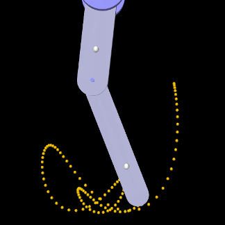
The following code fragment attaches a tracing probe to the last frame marker of the MultiJointedArm example of Section 3.5.16:
with the results shown in Figure 5.9 (left). To instead render the output as points, and with a coarser render interval of 0.02, one could modify the probe properties using
with the results shown in Figure 5.9 (right).

|
Tracing probes can also be created and edited interactively, as described in the section “Point Tracing” of the ArtiSynth User Interface Guide.
5.4.8 Position probes
Applications often find it useful to parametrically control the position of point or frame-based components, which include Point, Frame, FixedMeshBody, and their subclasses (e.g., Particle, RigidBody, and FemNode3d). This can be done by setting either the components’ position or targetPosition properties, and (for frame-based components) their orientation or targetOrientation properties. As described in Section 5.3.1.1, setting targetPosition and targetOrientation is often preferable as this will automatically update the component’s velocity, and so provide more information to the integrator, whereas setting position and orientation will leave the velocity unchanged.
When controlling the position and/or velocity of dynamic components, which include Point and Frame, it is important to ensure that their dynamic property is set to false and that they are unattached. Otherwise, the dynamic simulation will override any attempt at setting their position or velocity.
For frame-based components, the orientation and targetOrientation
properties describe their spatial orientation using an instance of
AxisAngle, which represents
a single rotation ![]() about a specific axis
about a specific axis ![]() in world coordinates (any
3D rotation can be expressed this way). However, when using this in a probe to
control or observe a frame-based component’s pose over time, a couple
of issues arise:
in world coordinates (any
3D rotation can be expressed this way). However, when using this in a probe to
control or observe a frame-based component’s pose over time, a couple
of issues arise:
-
•
There are other rotation representations that may be more useful or easier to specify, such as z-y-x or x-y-z rotations, in either radians or degrees.
-
•
Whatever rotation representation is used, care must be taken when interpolating it between knot points. Rotations cannot be treated as vectors and interpolation must instead take the form of curves on the 3D rotation group
 . The details are beyond the scope of this document but
were initially described by Shoemake [23].
. The details are beyond the scope of this document but
were initially described by Shoemake [23].
To address these issues, ArtiSynth supplies PositionInputProbe and PositionOutputProbe, which can be used to control or observe the position of one or more points or frame-based components, while offering a variety of rotation representations and handling rotation interpolation correctly. In particular, PositionInputProbes allow an application to supply key-frame animation control poses for frame-based components.
PositionInputProbes can be created with the constructors
In the above, name is the probe name (optional, can be null), and comp and comps refer to the component(s) to be assigned to the probe; as indicated above, these must be instances of Point, Frame, or FixedMeshBody. rotRep is an instance of RotationRep, which indicates how rotations should be represented, as described further below. The argument useTargetProps, if true, specifies that the probe should be attached to the targetPosition and (for frames) targetOrientation properties, vs. the position and orientation properties (if false). startTime and stopTime give the probe’s start and stop times, while filePath specifies a probe file from which to read in the probe’s basic parameters and data, per Section 5.4.4. Probes constructed without a file need to have data added, as per Section 5.4.5.
As indicated by the constructors, PositionInputProbes can control multiple
point and frame-based components, and this arrangement affects the size and
composition of the data vector. Each point component requires 3 numbers
specifying position, while each frame component requires ![]() numbers
specifying position and orientation, where
numbers
specifying position and orientation, where ![]() is the size of the
rotation representation. Although the orientation and targetOrientation properties describe rotation using an
AxisAngle, this will be converted
into knot point data based on the assigned RotationRep, with
is the size of the
rotation representation. Although the orientation and targetOrientation properties describe rotation using an
AxisAngle, this will be converted
into knot point data based on the assigned RotationRep, with ![]() equal to
either 3 or 4. The total size
equal to
either 3 or 4. The total size ![]() of the data vector is then
of the data vector is then
where ![]() is the number of points and
is the number of points and ![]() is the number of frames.
is the number of frames.
RotationRep provides a variety of ways to specify the rotation and applications can choose the most suitable:
- ZYX
-
Successive rotations, in radians, about the
 axes;
axes;  .
. - ZYX_DEG
-
Successive rotations, in degrees, about the
axes; . - XYZ
-
Successive rotations, in radians, about the
 axes; .
 - XYZ_DEG
-
Successive rotations, in degrees, about the
axes; . - AXIS_ANGLE
-
Axis-angle representation (
 ,
,  ), with the given in
radians;
), with the given in
radians;  . The axis does not need to be normalized.
 - AXIS_ANGLE_DEG
-
Axis-angle representation (
, ), with the given in
degrees; . The axis does not need to be normalized. - QUATERNION
-
Unit quaternion;
.
As a possibly more convenient alternative to the methods of Section 5.4.5, and to avoid having to explicitly pack the position and orientation information into the probe’s knot data, PositionInputProbes also supply the following methods to set the knot data for individual components being controlled by the probe:
| setPointData (Point point, double time, Vector3d pos) |
Set point position at a given time. |
| setFrameData (ModelComponent frame, double time, RigidTransform3d TFW) |
Set frame position/orientation at a given time. |
Each of these methods writes only the portion of the knot point at the indicated time that corresponds to the specified component; other portions are left unchanged or initialized to 0. For frames, TFW gives the pose (position/orientation) in the form of the transform from frame to world coordinates, and the orientation is transformed into knot point data according to the probe’s rotation representation.
PositionOutputProbes can be created with constructors analogous to PositionInputProbe:
The knot data format is the same as for PositionInputProbes, with rotations represented according to the setting of rotRep. There is no useTargetProps argument because PositionOutputProbes bind only to the position and orientation properties. If present, the filePath and interval arguments specify an attached file name for saving probe data and the update interval in seconds. Setting interval to -1 causes updating to occur at the simulation update rate, and this is the default for constructors without an interval argument.
5.4.9 Velocity probes
As with positions, applications may sometimes need to parametrically control or observe the velocity of point or frame-based components, which include Point, Frame, and their subclasses (but not FixedMeshBody, as this is not a dynamic component and so does not maintain a velocity). This can be done by setting either the components’ velocity or targetVelocity properties, with the latter sometimes preferable as it will automatically update the component’s position, whereas setting velocity will not. For frame-based components, velocity and targetVelocity are described by a 6-DOF Twist component that contains both translational and angular velocities. Unlike with finite rotations, there is only one representation for angular velocity (as a vector with units of radians/sec) and there are no interpolation issues.
When the position of a component is being controlled it is typically not necessary to also supply velocity information. This is especially true for position probes bound to targetPosition and targetOrientation properties, since these update velocity information automatically. However, for position probes bound to position and orientation, it can be sometimes be useful to use a velocity probe to also supply velocities. One example of this is when components are being tracked by inverse simulation (Chapter 10), as this extra information this can reduce tracking error and lag.
ArtiSynth provides VelocityInputProbe and VelocityOutputProbe to control or monitor the velocities of one or more point or frame-based components. The constructors for these are:
For all of these, the arguments are completely analogous to those for the constructors of PositionInputProbe and PositionOutputProbe, with the argument rotRep absent because it is not needed, and with useTargetProps specifying whether the probe should be attached to the targetVelocity or velocity properties.
If a position probe (either input or output) exists for a given collection of components, it is possible to automatically create a VelocityInputProbe for the same set of components, using one of the following static methods:
| VelocityInputProbe VelocityInputProbe.createNumeric (String name, NumericProbeBase source, double interval) |
Create by numeric differentiation. |
| VelocityInputProbe VelocityInputProbe.createInterpolated (String name, NumericProbeBase source, double interval) |
Create by interpolation. |
Both take an optional probe name and source probe. The update interval gives the time interval between the created knot points, with -1 causing this to be taken from the source. The first method creates the probe by numeric differentiation of the source’s position data and should be used only when the source’s data is dense, while the second method finds the derivative from the interpolation method of the source probe (as described by getInterpolationOrder()) and is better suited when the source data is sparse (although the resulting velocity will not be continuous unless the interpolation order is greater than linear).
The following code fragments creates a position probe and then uses this to generate a velocity probe:
5.4.10 Example: controlling a point and frame
 |
 |
A model demonstrating position and velocity probes is defined in
artisynth.demos.tutorial.PositionProbes
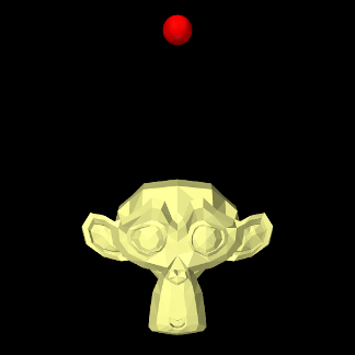
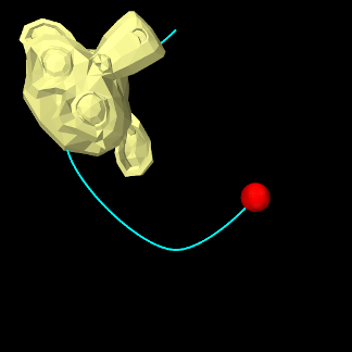
It creates a point and a rigid body (using the Blender monkey mesh), sets both to be non-dynamic, uses position and velocity probes to control their positions, and uses PositionOutputProbe and VelocityOutputProbe to monitor the resulting positions and velocities. The model class definition, excluding the import directives, is shown here:
The build() creates a MechModel and then adds to it a rigid body (created from the Blender monkey mesh) and a particle (lines 8-19). Both components are made non-dynamic to allow their positions and velocities to be controlled, and references to them are placed in a list used to create the probes (lines 21-24).
A PositionInputProbe for controlling the positions is created at lines 26-44, using a rotation representation of RotationRep.ZYX (successive rotations about the z-y-x axes, in radians). For this example, the useTargetProps is set to false (so that the probe binds to position and orientation), because we are going to be specifying velocities explicitly using another probe. Data for the probe is set using setData(), with the point and monkey positions/poses specified, in order, for times 0, 0.5, 1.0, 1.5 and 2. As per the rotation specification, poses for the monkey are given by 3 positions and 3 z-y-x rotations. Because the data is sparse, the probe’s interpolation order is set to Cubic to generate smooth motions.
A VelocityInputProbe is created by differentiating the position probe (lines 47-49); createInterpolated() is used because the position data is sparse and so numeric differentiation would yield bad results.
Finally, output probes to track both the resulting positions and velocities, together with a tracing probe to render the point’s path in cyan, are created at lines 51-65. When creating the PositionOutputProbe, we use the same rotation representation RotationRep.ZYX as for the input probe, but this is not necessary. For example, if one were to instead specify RotationRep.QUATERNION, then the frame orientations would be specified as quaternions.
To run this example in ArtiSynth, select All demos > tutorial > PositionProbes from the Models menu. When run, both the point and monkey will orbit around each other, with the point path being displayed by the tracing probe (Figure 5.10, right).
 |
 |
Several things about this demo should be noted:
-
•
The use of setData() in creating the position probe could be replaced by setPointData() and setFrameData(), as per
pip.setPointData (point, 0.5, new Point3d(-1.5,0,1.5));pip.setPointData (point, 1.0, new Point3d(0,0,0));pip.setPointData (point, 1.5, new Point3d(1.5,0,1.5));pip.setFrameData (monkey, 0.5, new RigidTransform3d(1.5,0,1.5, 0,PI/2,0));pip.setFrameData (monkey, 1.0, new RigidTransform3d(0.0,0,3.0, 0,PI,0));pip.setFrameData (monkey, 1.5, new RigidTransform3d(-1.5,0,1.5, 0,3*PI/2,0));Here, we can omit data for times 0 and 2 (at the probe’s start and end) because the motion begins and ends at the components’ initial positions, for which data was automatically added when the probe was created. (Likewise, data for times 0 and 2 could be omitted in the original code if addData() was used instead of setData()).
-
•
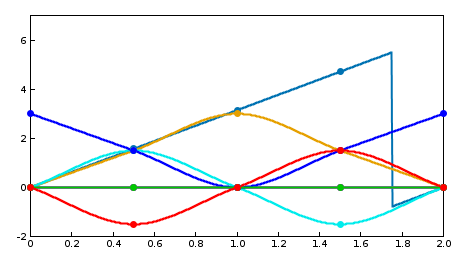
Position probes handle angle wrapping correctly. In the position input probe, the y-axis rotation for the monkey goes from
 to
to  between
  and
and  . However, by generating
“minimal distance” motions, interpolation proceeds as though the final angle
was specified as
. However, by generating
“minimal distance” motions, interpolation proceeds as though the final angle
was specified as  , allowing the circular motion to complete instead of
backtracking (although in the display plot, there is an apparent discontinuity
at
, allowing the circular motion to complete instead of
backtracking (although in the display plot, there is an apparent discontinuity
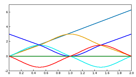
at  ; see Figure 5.11, left). Likewise, in
position output probes, as data is added, the rotation representation is
chosen to be as near as possible to the previous, so that in the
example the recorded
; see Figure 5.11, left). Likewise, in
position output probes, as data is added, the rotation representation is
chosen to be as near as possible to the previous, so that in the
example the recorded  rotation does indeed arrive at instead of
(Figure 5.11, right).
rotation does indeed arrive at instead of
(Figure 5.11, right). -
•
Since useTargetProps is set to false in the example, the velocity input probe is needed to set the component velocities; if this probe is made inactive (either in code or interactively in the timeline), then while the bodies will still move, no velocities will be set and the data in the velocity output probe will be uniformly 0.
Alternatively, if useTargetProps is set to true, then the input probes will be bound to targetPosition, targetOrientation, and targetVelocity, and both positions and velocities will be set for the components if either input probe is active. Reflecting the description in Section 5.3.1.1:
-
–
If the position input probe is active and the velocity input probe is inactive, then the velocities will be determined by differentiating the target position inputs (albeit with a one-step time lag).
-
–
If the position input probe is inactive and the velocity input probe is active, then the positions will be determined by integrating the target velocity inputs. Note that in this case, when the probes terminate, the components will continue moving with their last specified velocity.
-
–
If both the position and velocity input probes are active, then both the target position and velocity information will be used to update the component positions and velocities.
This provides a useful example of how target properties work.
-
–
5.4.11 Numeric monitor probes
In some cases, it may be useful for an application to deploy an output probe in which the data, instead of being collected from various component properties, is generated by a function within the probe itself. This ability is provided by a NumericMonitorProbe, which generates data using its generateData(vec,t,trel) method. This evaluates a vector-valued function of time at either the absolute time t or the probe-relative time trel and stores the result in the vector vec, whose size equals the vector size of the probe (as returned by getVsize()). The probe-relative time trel is determined by
| (5.0) |
where tstart and scale are the probe’s start time and scale factors as returned by getStartTime() and getScale().
As described further below, applications have several ways to control how a NumericMonitorProbe creates data:
-
•
Provide the probe with a DataFunction using the setDataFunction(func) method;
-
•
Override the generateData(vec,t,trel) method;
-
•
Override the apply(t) method.
The application is free to generate data in any desired way, and so in this sense a NumericMonitorProbe can be used similarly to a Monitor, with one of the main differences being that the data generated by a NumericMonitorProbe can be automatically displayed in the ArtiSynth GUI or written to a file.
The DataFunction interface declares an eval() method,
void eval (VectorNd vec, double t, double trel)
that for NumericMonitorProbes evaluates a vector-valued function of time, where the arguments take the same role as for the monitor’s generateData() method. Applications can declare an appropriate DataFunction and set or query it within the probe using the methods
The default implementation generateData() checks to see if a data function has been specified, and if so, uses that to generate the probe data. Otherwise, if the probe’s data function is null, the data is simply set to zero.
To create a NumericMonitorProbe using a supplied DataFunction, an application will create a generic probe instance, using one of its constructors such as
and then define and instantiate a DataFunction and pass it to the probe using setDataFunction(). It is not necessary to supply a file name (i.e., filePath can be null), but if one is provided, then the probe’s data can be saved to that file.
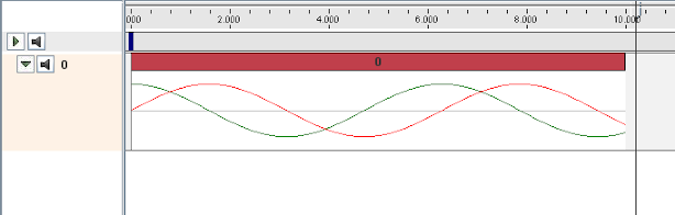
A complete example of this is defined in
artisynth.demos.tutorial.SinCosMonitorProbe
the listing for which is:
In this example, the DataFunction is implemented using the class SinCosFunction, which also implements Clonable and the associated clone() method. This means that the resulting probe will also be duplicatable within the GUI. Alternatively, one could implement SinCosFunction by extending DataFunctionBase, which implements Clonable by default. Probes containing DataFunctions which are not Clonable will not be duplicatable.
When the example is run, the resulting probe output is shown in the timeline image of Figure 5.12.
As an alternative to supplying a DataFunction to a generic NumericMonitorProbe, an application can instead subclass NumericMonitorProbe and override either its generateData(vec,t,trel) or apply(t) methods. As an example of the former, one could create a subclass as follows:
Note that when subclassing, one must also create constructor(s) for that subclass. Also, NumericMonitorProbes which don’t have a DataFunction set are considered to be clonable by default, which means that the clone() method may also need to be overridden if cloning requires any special handling.
5.4.12 Numeric control probes
In other cases, it may be useful for an application to deploy an input probe which takes numeric data, and instead of using it to modify various component properties, instead calls an internal method to directly modify the simulation in any way desired. This ability is provided by a NumericControlProbe, which applies its numeric data using its applyData(vec,t,trel) method. This receives the numeric input data via the vector vec and uses it to modify the simulation for either the absolute time t or probe-relative time trel. The size of vec equals the vector size of the probe (as returned by getVsize()), and the probe-relative time trel is determined as described in Section 5.4.11.
A NumericControlProbe is the Controller equivalent of a NumericMonitorProbe, as described in Section 5.4.11. Applications have several ways to control how they apply their data:
-
•
Provide the probe with a DataFunction using the setDataFunction(func) method;
-
•
Override the applyData(vec,t,trel) method;
-
•
Override the apply(t) method.
The application is free to apply data in any desired way, and so in this sense a NumericControlProbe can be used similarly to a Controller, with one of the main differences being that the numeric data used can be automatically displayed in the ArtiSynth GUI or read from a file.
The DataFunction interface declares an eval() method,
void eval (VectorNd vec, double t, double trel)
that for NumericControlProbes applies the numeric data, where the arguments take the same role as for the monitor’s applyData() method. Applications can declare an appropriate DataFunction and set or query it within the probe using the methods
The default implementation applyData() checks to see if a data function has been specified, and if so, uses that to apply the probe data. Otherwise, if the probe’s data function is null, the data is simply ignored and the probe does nothing.
To create a NumericControlProbe using a supplied DataFunction, an application will create a generic probe instance, using one of its constructors such as
and then define and instantiate a DataFunction and pass it to the probe using setDataFunction(). The latter constructor creates the probe and reads in both the data and timing information from the specified file.
A complete example of this is defined in
artisynth.demos.tutorial.SpinControlProbe
the listing for which is:
This example creates a simple box and then uses a NumericControlProbe to spin it about the ![]() axis, using a DataFunction implementation called SpinFunction. A clone method
is also implemented to ensure that the probe will be duplicatable in
the GUI, as described in Section 5.4.11. A
single channel of data is used to control the orientation angle of the
box about
axis, using a DataFunction implementation called SpinFunction. A clone method
is also implemented to ensure that the probe will be duplicatable in
the GUI, as described in Section 5.4.11. A
single channel of data is used to control the orientation angle of the
box about ![]() , as shown in Figure 5.13.
, as shown in Figure 5.13.
Alternatively, an application can subclass NumericControlProbe and override either its applyData(vec,t,trel) or apply(t) methods, as described for NumericMonitorProbes (Section 5.4.11).
![[LOGO]](data:image/png;base64,iVBORw0KGgoAAAANSUhEUgAAAAsAAAAOCAYAAAD5YeaVAAAAAXNSR0IArs4c6QAAAAZiS0dEAP8A/wD/oL2nkwAAAAlwSFlzAAALEwAACxMBAJqcGAAAAAd0SU1FB9wKExQZLWTEaOUAAAAddEVYdENvbW1lbnQAQ3JlYXRlZCB3aXRoIFRoZSBHSU1Q72QlbgAAAdpJREFUKM9tkL+L2nAARz9fPZNCKFapUn8kyI0e4iRHSR1Kb8ng0lJw6FYHFwv2LwhOpcWxTjeUunYqOmqd6hEoRDhtDWdA8ApRYsSUCDHNt5ul13vz4w0vWCgUnnEc975arX6ORqN3VqtVZbfbTQC4uEHANM3jSqXymFI6yWazP2KxWAXAL9zCUa1Wy2tXVxheKA9YNoR8Pt+aTqe4FVVVvz05O6MBhqUIBGk8Hn8HAOVy+T+XLJfLS4ZhTiRJgqIoVBRFIoric47jPnmeB1mW/9rr9ZpSSn3Lsmir1fJZlqWlUonKsvwWwD8ymc/nXwVBeLjf7xEKhdBut9Hr9WgmkyGEkJwsy5eHG5vN5g0AKIoCAEgkEkin0wQAfN9/cXPdheu6P33fBwB4ngcAcByHJpPJl+fn54mD3Gg0NrquXxeLRQAAwzAYj8cwTZPwPH9/sVg8PXweDAauqqr2cDjEer1GJBLBZDJBs9mE4zjwfZ85lAGg2+06hmGgXq+j3+/DsixYlgVN03a9Xu8jgCNCyIegIAgx13Vfd7vdu+FweG8YRkjXdWy329+dTgeSJD3ieZ7RNO0VAXAPwDEAO5VKndi2fWrb9jWl9Esul6PZbDY9Go1OZ7PZ9z/lyuD3OozU2wAAAABJRU5ErkJggg==)