3.3 Mesh components
ArtiSynth models frequently incorporate 3D mesh geometry, as defined by the geometry classes PolygonalMesh, PolylineMesh, and PointMesh described in Section 2.5. Within a model, these basic classes are typically enclosed within container components that are subclasses of MeshComponent. Commonly used instances of these include
- RigidMeshComp
-
Introduced in Section 3.2.9, these contain the mesh geometry for rigid bodies, and are stored in a rigid body subcomponent list named meshes. Their mesh vertex positions are fixed with respect to their body’s coordinate frame.
- FemMeshComp
-
Contain mesh geometry associated with finite element models (Chapter 6), including surfaces meshes and embedded mesh geometry, and are stored in a subcomponent list of the FEM model named meshes. Their mesh vertex positions change as the FEM model deforms.
- SkinMeshBody
-
Described in detail in Chapter 11, these describe “skin” geometry that encloses both rigid bodies and/or FEM models. Their mesh vertex positions change as the underlying bodies move and deform. Skinning meshes may be placed anywhere, but are typically stored in the meshBodies component list of a MechModel.
- FixedMeshBody
-
Described further below, these store arbitrary mesh geometry (polygonal, polyline, and point) and provide (like rigid bodies) a rigid coordinate frame that allows the mesh to be positioned and oriented arbitrarily. As their name suggests, their mesh vertex positions are fixed with respect to this coordinate frame. Fixed body meshes may be placed anywhere, but are typically stored in the meshBodies component list of a MechModel.
3.3.1 Fixed mesh bodies
As mentioned above, FixedMeshBody can be used for placing arbitrary mesh geometry within an ArtiSynth model. These mesh bodies are non-dynamic: they do not interact or collide with other model components, and they function primarily as 3D graphical objects. They can be created from primary mesh components using constructors such as:
| FixedMeshBody (MeshBase mesh) |
Create an unnamed body containing a specified mesh. |
| FixedMeshBody (String name, MeshBase mesh) |
Create a named body containing a specified mesh. |
It should be noted that the primary meshes are not copied and are instead stored by reference, and so any subsequent changes to them will be reflected in the mesh body. As with rigid bodies, fixed mesh bodies contain a coordinate frame, or pose, that describes the position and orientation of the body with respect to world coordinates. Methods to control the pose include:
| RigidTransform3d getPose() |
Returns the pose of the body (with respect to world). |
| void setPose (RigidTransform3d XFrameToWorld) |
Sets the pose of the body. |
| Point3d getPosition() |
Returns the body position (pose translation component). |
| void setPosition (Point3d pos) |
Sets the body position. |
| AxisAngle getOrientation() |
Returns the body orientation (pose rotation component). |
| void setOrientation (AxisAngle axisAng) |
Sets the body orientation. |
Once created, a canonical place for storing mesh bodies is the MechModel component list meshBodies. Methods for maintaining this list include:
| ComponentListView<MeshComponent> meshBodies() |
Returns the meshBodies list. |
| void addMeshBody (MeshComponent mcomp) |
Adds mcomp to meshBodies. |
| boolean removeMeshBody (MeshComponent mcomp) |
Removes mcomp from meshBodies. |
| void clearMeshBodies() |
Clears the meshBodies list. |
Meshes used for instantiating fixed mesh bodies are typically read from files (Section 2.5.5), but can also be created using factory methods (Section 2.5.1). As an example, the following code fragment creates a torus mesh using a factory method, set its pose, and then adds it to a MechModel:
Rendering of mesh bodies is controlled using the same properties described in Section 3.2.8 for rigid bodies, including the renderProps subproperties faceColor, shading, alpha, faceStyle, and drawEdges, and the properties axisLength and axisDrawStyle for displaying a body’s coordinate frame.
3.3.2 Example: adding mesh bodies to MechModel
A simple application that creates a pair of fixed meshes and adds them to a MechModel is defined in
artisynth.demos.tutorial.FixedMeshes
The build() method for this is shown below:
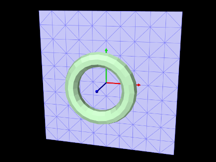
After creating a MechModel (lines 3-4), a torus shaped mesh is imported from the file data/torus_9_24.obj (lines 8-16). As described in Section 2.6, the RootModel method getSourceRelativePath() is used to locate this file relative to the model’s source folder. The file path is used in the PolygonalMesh constructor, which is enclosed within a try/catch block to handle possible I/O exceptions. Once imported, the mesh is used to instantiate a FixedMeshBody named "torus" which is added to the MechModel (lines 18-19).
Another mesh, representing a square, is created with a factory method
and used to instantiate a mesh body named "square" (lines
22-26). The factory method specifies both the size and triangle
density of the mesh in the ![]() -
-![]() plane. Once created, the square’s
pose is set to a 90 degree rotation about the
plane. Once created, the square’s
pose is set to a 90 degree rotation about the ![]() axis and a
translation of 0.5 along
axis and a
translation of 0.5 along ![]() (lines 28-29).
(lines 28-29).
Rendering properties are set at lines 33-41. The torus is made pale green by setting its face color; the coordinate frame for the square is made visible as solid arrows using the axisLength and axisDrawStyle properties; and the square is made blue gray, with its edges made visible and drawn using a darker color, and its face style set to FRONT_AND_BACK so that it’s visible from either side.
To run this example in ArtiSynth, select All demos > tutorial > FixedMeshes from the Models menu. The model should load and initially appear as in Figure 3.8.
![[LOGO]](data:image/png;base64,iVBORw0KGgoAAAANSUhEUgAAAAsAAAAOCAYAAAD5YeaVAAAAAXNSR0IArs4c6QAAAAZiS0dEAP8A/wD/oL2nkwAAAAlwSFlzAAALEwAACxMBAJqcGAAAAAd0SU1FB9wKExQZLWTEaOUAAAAddEVYdENvbW1lbnQAQ3JlYXRlZCB3aXRoIFRoZSBHSU1Q72QlbgAAAdpJREFUKM9tkL+L2nAARz9fPZNCKFapUn8kyI0e4iRHSR1Kb8ng0lJw6FYHFwv2LwhOpcWxTjeUunYqOmqd6hEoRDhtDWdA8ApRYsSUCDHNt5ul13vz4w0vWCgUnnEc975arX6ORqN3VqtVZbfbTQC4uEHANM3jSqXymFI6yWazP2KxWAXAL9zCUa1Wy2tXVxheKA9YNoR8Pt+aTqe4FVVVvz05O6MBhqUIBGk8Hn8HAOVy+T+XLJfLS4ZhTiRJgqIoVBRFIoric47jPnmeB1mW/9rr9ZpSSn3Lsmir1fJZlqWlUonKsvwWwD8ymc/nXwVBeLjf7xEKhdBut9Hr9WgmkyGEkJwsy5eHG5vN5g0AKIoCAEgkEkin0wQAfN9/cXPdheu6P33fBwB4ngcAcByHJpPJl+fn54mD3Gg0NrquXxeLRQAAwzAYj8cwTZPwPH9/sVg8PXweDAauqqr2cDjEer1GJBLBZDJBs9mE4zjwfZ85lAGg2+06hmGgXq+j3+/DsixYlgVN03a9Xu8jgCNCyIegIAgx13Vfd7vdu+FweG8YRkjXdWy329+dTgeSJD3ieZ7RNO0VAXAPwDEAO5VKndi2fWrb9jWl9Esul6PZbDY9Go1OZ7PZ9z/lyuD3OozU2wAAAABJRU5ErkJggg==)