3.4 Joints and connectors
In a typical mechanical model, many of the rigid bodies are interconnected, either using spring-type components that exert binding forces on the bodies, or through joints and connectors that enforce the connection using hard constraints. This section describes the latter. While the discussion focuses on rigid bodies, joints and connectors can be used more generally with any body that implements the ConnectableBody interface. In particular, this allows joints to also interconnect finite element models, as described in Section 6.6.4.
3.4.1 Joints and coordinate frames
Consider two rigid bodies A and B. The pose of body B with respect to
body A can be described by the 6 DOF rigid transform ![]() . If A
and B are unconnected,
. If A
and B are unconnected, ![]() may assume any possible value and has
a full six degrees of freedom. A joint between A and B
constrains the set of poses that are possible between the two bodies
and reduces the degrees of freedom available to
may assume any possible value and has
a full six degrees of freedom. A joint between A and B
constrains the set of poses that are possible between the two bodies
and reduces the degrees of freedom available to ![]() . For ease
of use, the constraining action of a joint is described with respect
to a pair of local coordinate frames C and D that are connected to
frames A and B, respectively, by auxiliary transformations. This
allows joints to be placed at locations that do not correspond
directly to frames A or B.
. For ease
of use, the constraining action of a joint is described with respect
to a pair of local coordinate frames C and D that are connected to
frames A and B, respectively, by auxiliary transformations. This
allows joints to be placed at locations that do not correspond
directly to frames A or B.
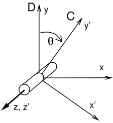
The joint frames C and D move with respect to each other as the joint
moves. The allowed joint motions therefore correspond to the allowed
values of the joint transform ![]() . Although both frames
typically move with their attached bodies, D is considered the base frame and C the motion frame (this is because when a joint
is used to connect a single body to ground, body B is set to null and the world frame takes its place). As an example of a
joint’s constraining effect, consider a hinge joint (Figure
3.9), which allows C to move with respect to D only by
rotating about the
. Although both frames
typically move with their attached bodies, D is considered the base frame and C the motion frame (this is because when a joint
is used to connect a single body to ground, body B is set to null and the world frame takes its place). As an example of a
joint’s constraining effect, consider a hinge joint (Figure
3.9), which allows C to move with respect to D only by
rotating about the ![]() axis while the origins of C and D remain
coincident. Other motions are prohibited. If we let
axis while the origins of C and D remain
coincident. Other motions are prohibited. If we let ![]() describe
the counter-clockwise rotation angle of C about the
describe
the counter-clockwise rotation angle of C about the ![]() axis, then
axis, then
![]() should always have the form
should always have the form
 |
(3.1) |
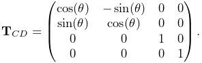
When a joint is attached to bodies A and B, frame C is fixed to body A
and frame D is fixed to body B. Except in special cases, the joint
frames C and D are not coincident with the body frames A
and B. Instead, they are located relative to A and B by the
transforms ![]() and
and ![]() , respectively
(Figure 3.10). Since
, respectively
(Figure 3.10). Since ![]() and
and ![]() are
both fixed, the joint constraints on
are
both fixed, the joint constraints on ![]() constrain the relative
poses of A and B, with
constrain the relative
poses of A and B, with ![]() determined from
determined from
| (3.2) |
(See Section A.2 for a discussion of determining transforms between related coordinate frames).
3.4.2 Joint coordinates, constraints, and errors
Each different joint and connector type restricts the motion between
two bodies to ![]() degrees of freedom, for some
degrees of freedom, for some ![]() . Sometimes,
the joint also defines a set of
. Sometimes,
the joint also defines a set of ![]() coordinates that parameterize
these
coordinates that parameterize
these ![]() DOFs. For example, the hinge joint described above is
parameterized by
DOFs. For example, the hinge joint described above is
parameterized by ![]() . Other examples are given in
Section 3.5: a 2 DOF cylindrical has coordinates
. Other examples are given in
Section 3.5: a 2 DOF cylindrical has coordinates ![]() and
and ![]() , a 3 DOF gimbal joint is parameterized by the
roll-pitch-yaw angles
, a 3 DOF gimbal joint is parameterized by the
roll-pitch-yaw angles ![]() ,
, ![]() , and
, and ![]() , etc. When
, etc. When
![]() (where
(where ![]() is the identity transform), the coordinates
are usually all equal to zero, and the joint is said to be in the zero state.
is the identity transform), the coordinates
are usually all equal to zero, and the joint is said to be in the zero state.
As explained in Section 1.2.3, ArtiSynth uses a
full coordinate formulation for dynamic simulation. That means that
instead of using joint coordinates to describe system state, it uses
the combined full coordinates ![]() of all dynamic components. For
example, a model consisting of a single rigid body connected to ground
by a hinge joint will have 6 DOF (corresponding to the 6 DOF of the
body), rather than the 1 DOF implied by the hinge joint. The DOF
restrictions imposed by the joints are then enforced by a set of
linearized constraint relationships
of all dynamic components. For
example, a model consisting of a single rigid body connected to ground
by a hinge joint will have 6 DOF (corresponding to the 6 DOF of the
body), rather than the 1 DOF implied by the hinge joint. The DOF
restrictions imposed by the joints are then enforced by a set of
linearized constraint relationships
| (3.3) |
that restrict the body velocities ![]() computed at each simulation
step, usually by solving an MLCP like (1.13). As
explained in Section 1.2.3, the right side
vectors
computed at each simulation
step, usually by solving an MLCP like (1.13). As
explained in Section 1.2.3, the right side
vectors ![]() and
and ![]() in (3.3) contain time
derivative terms, which for simplicity much of the following
presentation will assume to be 0.
in (3.3) contain time
derivative terms, which for simplicity much of the following
presentation will assume to be 0.
Each joint contributes its own set of constraint equations to (3.3). Typically these take the form of bilateral, or equality, constraints
| (3.4) |
which are added to the system’s global bilateral constraint matrix
![]() .
. ![]() contains
contains ![]() rows providing
rows providing ![]() individual
constraints
individual
constraints ![]() .
During simulation, these give rise to
.
During simulation, these give rise to ![]() constraint
forces (corresponding to
constraint
forces (corresponding to ![]() in (1.10))
which enforce the constraints.
in (1.10))
which enforce the constraints.
In some cases, the joint also maintains unilateral, or inequality
constraints, to keep ![]() out of inadmissible regions. These take
the form
out of inadmissible regions. These take
the form
| (3.5) |
and are added to the system’s global unilateral constraint matrix
![]() . They give rise to constraint forces corresponding to
. They give rise to constraint forces corresponding to ![]() in
(1.10). A common use of unilateral constraints
is to enforce range limits of the joint coordinates (Section
3.4.5), such as
in
(1.10). A common use of unilateral constraints
is to enforce range limits of the joint coordinates (Section
3.4.5), such as
| (3.6) |
A specific unilateral constraint is added to ![]() only when
only when
![]() is on or within the boundary of the inadmissible region
associated with that constraint. The constraint is then said to be
engaged. The combined number of bilateral and engaged unilateral
constraints for a particular joint should not exceed 6; otherwise, the
joint would be overconstrained.
is on or within the boundary of the inadmissible region
associated with that constraint. The constraint is then said to be
engaged. The combined number of bilateral and engaged unilateral
constraints for a particular joint should not exceed 6; otherwise, the
joint would be overconstrained.
Joint coordinates, when supported for a particular joint, can be both
read and set. Setting a coordinate causes the joint transform
![]() to change. To accommodate this, the system adjusts the poses
of one or both bodies connected to the joint, along with adjacent
bodies connected to them, with preference given to bodies that are not
attached to “ground”. However, if this is done during simulation,
and particularly if one or both of the bodies connected to the joint
are moving dynamically, the results will be unpredictable and will
likely conflict with the simulation.
to change. To accommodate this, the system adjusts the poses
of one or both bodies connected to the joint, along with adjacent
bodies connected to them, with preference given to bodies that are not
attached to “ground”. However, if this is done during simulation,
and particularly if one or both of the bodies connected to the joint
are moving dynamically, the results will be unpredictable and will
likely conflict with the simulation.
Joint coordinates are also often exported as properties. For example,
the
HingeJoint
class (Section 3.5) exports its ![]() coordinate
as the property theta, which can be accessed in the GUI, or via
the accessor methods
coordinate
as the property theta, which can be accessed in the GUI, or via
the accessor methods
Since joint constraints are generally nonlinear, their linearized
enforcement at the velocity level by (3.3) will
usually produce small errors as the simulation proceeds. These errors
are reduced using a position correction step described in
Section 4.9.1 and [11].
Errors can also be caused by joint compliance
(Section 3.4.9). Both effects mean that the joint
transform ![]() may deviate from the allowed values dictated by
the joint type. In ArtiSynth, this is accounted for by introducing an
additional constraint frame G between D and C
(Figure 3.11). G is computed to be the nearest frame
to C that lies exactly in the joint constraint space.
may deviate from the allowed values dictated by
the joint type. In ArtiSynth, this is accounted for by introducing an
additional constraint frame G between D and C
(Figure 3.11). G is computed to be the nearest frame
to C that lies exactly in the joint constraint space. ![]() is
therefore a valid joint transform,
is
therefore a valid joint transform, ![]() accommodates the error,
and the whole joint transform is given by the composition
accommodates the error,
and the whole joint transform is given by the composition
| (3.7) |
If there is no compliance or joint error, then frames G and C are
identical, ![]() , and
, and ![]() . Because
. Because ![]() describes the joint error, we sometimes refer to it as
describes the joint error, we sometimes refer to it as ![]() .
.

3.4.3 Creating joints
Joint and connector components in ArtiSynth are both derived from the superclass BodyConnector, with joints being further derived from JointBase, which provides support for coordinates. Some of the commonly used joints and connectors are described in Section 3.5.
An application creates a joint by constructing it and adding it to a MechModel. For this, two things need to be specified:
-
1.
The bodies A and B being connected;
-
2.
The initial locations of the C and D frames.
For the second item, it is often more convenient to specify C and D in world
coordinates, i.e., as ![]() and
and ![]() , and then determine
, and then determine ![]() and
and
![]() from
from
| (3.8) | ||||
| (3.9) |
where ![]() and
and ![]() are the current poses of A and B.
are the current poses of A and B.
Many joints have constructors of the form
which specifies only ![]() and the bodies A and B. The constructor
then computes
and the bodies A and B. The constructor
then computes ![]() from
from
| (3.10) |
where ![]() is the joint’s initial
is the joint’s initial ![]() value returned by
getCurrentTCD(). For joints
with coordinates, the initial
value returned by
getCurrentTCD(). For joints
with coordinates, the initial ![]() is determined from the initial
coordinate values (which are usually 0). Typically (but not always), the
initial
is determined from the initial
coordinate values (which are usually 0). Typically (but not always), the
initial ![]() is also the identity, so that
is also the identity, so that ![]() .
.
After the joint is created, it should be added to the system’s MechModel using addBodyConnector(), as shown in the following code fragment:
Joints usually offer a number of other constructors that let its world location and body relationships to be specified in different ways. These may include:
The first, which is restricted to rigid bodies, allows the application
to explicitly specify transforms ![]() and
and ![]() connecting
frames C and D to the body frames A and B, and is useful when
connecting
frames C and D to the body frames A and B, and is useful when
![]() and
and ![]() are explicitly known, or the initial value of
are explicitly known, or the initial value of
![]() is not the identity. Likewise, the second constructor
allows
is not the identity. Likewise, the second constructor
allows ![]() and
and ![]() to be explicitly specified, with
to be explicitly specified, with
![]() if
if ![]() . For instance, suppose
. For instance, suppose
![]() and
and ![]() are both known. Then we can use the
relationship
are both known. Then we can use the
relationship
| (3.11) |
to create the joint as in the following code fragment:
As an alternative to specifying ![]() or its equivalents, some
joint types provide constructors that let the application locate
specific joint features. These may be easier to use in some cases. For
instance, HingeJoint provides a
constructor
or its equivalents, some
joint types provide constructors that let the application locate
specific joint features. These may be easier to use in some cases. For
instance, HingeJoint provides a
constructor
that specifies origin of D and its ![]() axis (which is the rotation
axis), with the remaining orientation of D aligned as closely as
possible with the world.
SphericalJoint provides a
constructor
axis (which is the rotation
axis), with the remaining orientation of D aligned as closely as
possible with the world.
SphericalJoint provides a
constructor
that specifies origin of D and aligns its orientation with the world. Users should consult the source code or API documentation for specific joints to see what special constructors may be available.
It is also possible to use a joint to connect a single body to “ground” (i.e., the world frame). When this is done, the body in question is always bodyA, and bodyB is null. Most joints provide a constructor of the form
which allows this to be done explicitly. Alternatively, most joint constructors which supply body B will allow this to be specified as null, so that body A will be connected to ground by default.
When using joints to build an articulated structure, the usual convention is for bodyA to be on the distal, or “outer”, side of the joint and for bodyB to be on the proximal, or “inner”, side.
Finally, it is also possible to create a joint using its default constructor and attach it to the bodies afterward, using the various setBodies() methods:
| void setBodies (ConnectableBody bodyA, ConnectableBody bodyB, RigidTransform3d TDW) |
Set A and B given TDW. |
| void setBodies (ConnectableBody bodyA, ConnectableBody bodyB, RigidTransform3d TCW, RigidTransform3d TDW) |
Set A and B given TCW and TDW. |
| void setBodies (RigidBody bodyA, RigidTransform3d TCA, RigidBody bodyB, RigidTransform3d TDB) |
Set A and B given TCA and TDB. |
| void setBodies (ConnectableBody bodyA, FrameAttachment attachmentA, ConnectableBody bodyB, FrameAttachment attachmentB) |
Set A and B with custom attachments. |
| void setBodyA (ConnectableBody bodyA, RigidTransform3d TCW) |
Set A given TCW. |
| void setBodyA (ConnectableBody bodyA, FrameAttachment attachmentA) |
Set A with custom attachment. |
| void setBodyB (ConnectableBody bodyB, RigidTransform3d TDW) |
Set B given TDW. |
| void setBodyB (ConnectableBody bodyB, FrameAttachment attachmentB) |
Set B with custom attachment. |
As with the constructors, TDW and TCW give the locations of D and C in world coordinates, and if TCW is needed but not specified, it is computed per equation (3.10). bodyB can also be given as null, which will cause body A to be attached to ground. The methods specifying FrameAttachments allow for situations where special attachment types are needed, such as when connecting joints to finite element models (Section 6.6.4). The setBodyA() and setBodyB() methods connect body A (or body B) while leaving body B (or body A) alone, and are useful when it is necessary to set (or reset) only one body connection.
The following example creates a HingeJoint using setBodies():
A more complicated, but exactly equivalent, version using setBodyA() and setBodyB() is given by
One reason for using setBodies() is that it allows the joint transform
![]() to be modified (by setting coordinate values) before setBodies() is called; this is discussed further in
Section 3.4.4.
to be modified (by setting coordinate values) before setBodies() is called; this is discussed further in
Section 3.4.4.
3.4.4 Working with coordinates
As mentioned in Section 3.4.2, some joints
support coordinates that parameterize the valid motions within the
joint transform ![]() . All such joints are subclasses of
JointBase,
which provides some generic methods for querying and setting
coordinate values (JointBase is in turn a subclass of
BodyConnector).
. All such joints are subclasses of
JointBase,
which provides some generic methods for querying and setting
coordinate values (JointBase is in turn a subclass of
BodyConnector).
The number of coordinates is returned by the method numCoordinates(); if this returns 0, then coordinates are not
supported. Each coordinate has an index in the range ![]() ,
where
,
where ![]() is the number of coordinates. Coordinate values can be
queried or set using the following methods:
is the number of coordinates. Coordinate values can be
queried or set using the following methods:
Specific joint types usually also provide names for their joint
coordinates, along with integer constants describing their indices
and methods for accessing their values. For example,
CylindricalJoint
supports two coordinates, ![]() and
and ![]() , along with
the following:
, along with
the following:
The coordinate values are also exported as the properties z and theta, allowing them to be set in the GUI. For convenience, particularly in GUI applications, the properties and methods for controlling specific angular coordinates generally use degrees instead of radians.
It is recommended to call setCoordinate methods only after a joint has been added to its MechModel, in order to ensure that other bodies in its articulated structure, together with any muscle wrap paths (Chapter 9), are updated appropriately.
As discussed in Section 3.4.2, unlike in some multibody simulation systems (such as OpenSim), joint coordinates are not fundamental quantities that describe system state. As such, then, coordinates can usually only be set in specific circumstances that avoid simulation conflicts. In general, when joint coordinates are set, the system adjusts the poses of one or both bodies connected to this joint, along with adjacent bodies connected to them, with preference given to bodies that are not attached to “ground”. However, if this is done during simulation, and particularly if one or both of the bodies connected to the joint are moving dynamically, the results will be unpredictable and will likely conflict with the simulation.
Coordinate setting is discussed in greater detail in Section 3.6, along with the CoordinateSetter class that can be used to set coordinate values across several joints simultaneously.
If a joint has been created with its default constructor and not yet
attached to any bodies, then setting joint values will simply set the
joint transform ![]() . This can be useful in situations where one
needs to initialize a joint’s
. This can be useful in situations where one
needs to initialize a joint’s ![]() to a non-identity value
corresponding to a particular set of joint coordinates:
to a non-identity value
corresponding to a particular set of joint coordinates:
This can also be done in vector form:
In either of these cases, setBodies() will not use ![]() but instead use the value determined by the initial coordinate
values.
but instead use the value determined by the initial coordinate
values.
To determine the ![]() corresponding to a particular set of
coordinates, one may use the method
corresponding to a particular set of
coordinates, one may use the method
In some cases, within a model’s build() method, one may wish to set initial coordinates after a joint has been attached to its bodies, in order to move those bodies (along with the bodies attached to them) into an initial configuration without having to explicitly calculate the poses from the joint coordinates. As mentioned above, the system will make a decision about which attached bodies are most “free” and adjust their poses accordingly. This is done in the example of the next section.
3.4.5 Coordinate limits and locking
It is possible to set limits on a joint coordinate’s range, and also to lock a coordinate in place at its current value.
When a joint coordinate hits either an upper or lower range limit, a unilateral constraint is invoked to prevent it from violating the limit, and remains engaged until the joint moves away from the limit. Each range constraint that is engaged reduces the number of joint DOFs by one.
By default, joint range limits are usually disabled (i.e., they are
set to ![]() ). They can be queried and set, for a given
joint with index idx, using the methods:
). They can be queried and set, for a given
joint with index idx, using the methods:
where range limits for angular coordinates are specified in radians. For convenience, the following methods are also provided which use degrees instead of radians for angular coordinates:
Range checking can be disabled by setting the range to
![]() , or by specifying rng as null, which
implicitly does the same thing.
, or by specifying rng as null, which
implicitly does the same thing.
Ranges for angular coordinates are not limited to
but can instead be set to larger values; the joint will continue to wrap until the limit is reached.
Joint coordinates can also be locked, so that they hold their current value and don’t move. A joint is locked using a bilateral constraint that prevents motion in either direction and reduces the joint’s DOF count by one. The following methods are available for querying or setting a coordinate’s locked status:
As with coordinate values, specific joint types usually provide methods for controlling the ranges and locking status of individual coordinates, with ranges for angular coordinates specified in degrees instead of radians. For example, CylindricalJoint supplies the methods
The range and locking information is also exported as the properties zRange, thetaRange, zLocked, and thetaLocked, allowing them to be set in the GUI.
3.4.6 Example: a simple hinge joint
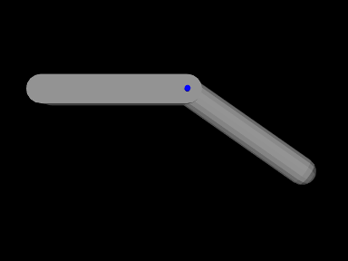
A simple model showing two rigid bodies connected by a joint is defined in
artisynth.demos.tutorial.RigidBodyJoint
The build method for this model is given below:
A MechModel is created as usual at line 4. However, in this
example, we also set some parameters for it:
setGravity() is
used to set the gravity acceleration vector to ![]() instead
of the default value of
instead
of the default value of ![]() , and the frameDamping
and rotaryDamping properties (Section
3.2.7) are set to provide appropriate damping.
, and the frameDamping
and rotaryDamping properties (Section
3.2.7) are set to provide appropriate damping.
Each of the two rigid bodies are created from a mesh and a density. The meshes themselves are created using the factory methods MeshFactory.createRoundedBox() and MeshFactory.createRoundedCylinder() (lines 13 and 22), and then RigidBody.createFromMesh() is used to turn these into rigid bodies with a density of 0.2 (lines 17 and 25). The pose of the two bodies is set using RigidTransform3d objects created with x, y, z translation and axis-angle orientation values (lines 18 and 26).
The hinge joint is implemented using HingeJoint, which is constructed at line 32 with the joint coordinate frame D being located in world coordinates by TDW as described in Section 3.4.3.
Once the joint is created and added to the MechModel, the method
setTheta() is
used to explicitly set the joint parameter to 35 degrees. The joint
transform ![]() is then set appropriately and bodyA is moved
to accommodate this (bodyA being chosen since it is the most
free to move).
is then set appropriately and bodyA is moved
to accommodate this (bodyA being chosen since it is the most
free to move).
Finally, joint rendering properties are set starting at line 42. We render the joint as a cylindrical shaft about the rotation axis, using its shaftLength and shaftRadius properties. Joint rendering is discussed in more detail in Section 3.4.11).
3.4.7 Joint coordinate handles
The class JointCoordinateHandle is a convenience class that encapsulates access to a single coordinate by containing both its joint and index within that joint. It can be easily constructed as follows,
and offers a number of methods to directly access coordinate properties:
| double getValue() |
Returns the value (in radians for rotary coordinates). |
| double getValueDeg() |
Returns the value (in degrees for rotary coordinates). |
| String getName() |
Queries the coordinate’s name. |
| JointBase getJoint() |
Returns the coordinate’s joint. |
| int getIndex() |
Queries the coordinate’s index within the joint. |
| MotionType getMotionType() |
Queries the coordinate’s motion type. |
| DoubleInterval getValueRange() |
Returns the range (in radians for rotary coordinates). |
| void setValueRange(DoubleInterval range) |
Sets the range (in radians for rotary coordinates). |
| DoubleInterval getValueRangeDeg() |
Returns the coordinate’s range (in degrees for rotary coordinates). |
| void setValueRangeDeg(DoubleInterval range) |
Sets the range (in degrees for rotary coordinates). |
| boolean isLocked() |
Queries whether the coordinate is locked. |
| void setLocked (boolean locked) |
Sets whether the coordinate is locked. |
3.4.8 Constraint forces
During each simulation solve step, the joint velocity constraints
described by (3.4) and (3.5) are
enforced by bilateral and unilateral constraint forces ![]() and
and
![]() :
:
| (3.11) |
Here, ![]() and
and ![]() are spatial forces (or wrenches, Section
A.5) acting in the joint coordinate
frame C, and
are spatial forces (or wrenches, Section
A.5) acting in the joint coordinate
frame C, and ![]() and
and ![]() are the Lagrange multipliers
computed as part of the mechanical system solve (see
(1.13) and (1.10)). The sizes
of
are the Lagrange multipliers
computed as part of the mechanical system solve (see
(1.13) and (1.10)). The sizes
of ![]() and
and ![]() equal the number of bilateral and engaged unilateral constraints in the joint; these numbers can be
queried for a particular joint using the methods
numBilateralConstraints()
and
numEngagedUnilateralConstraints().
(The number of engaged unilateral constraints may be less than the
total number of unilateral constraints; the latter may be queried with
numUnilateralConstraints(),
while the total number of
constraints is returned by
numConstraints().
equal the number of bilateral and engaged unilateral constraints in the joint; these numbers can be
queried for a particular joint using the methods
numBilateralConstraints()
and
numEngagedUnilateralConstraints().
(The number of engaged unilateral constraints may be less than the
total number of unilateral constraints; the latter may be queried with
numUnilateralConstraints(),
while the total number of
constraints is returned by
numConstraints().
Applications may sometimes need to query the current constraint force values, typically from within a controller or monitor (Section 5.3). The Lagrange multipliers themselves may be obtained with
which load the multipliers into lam or the and set their sizes to the number of bilateral or engaged unilateral constraints. Alternatively, one can retrieve the individual multiplier for the constraint indexed by idx using
Typically, it is more useful to find the spatial constraint forces
![]() and
and ![]() , which can be obtained with respect to frame C:
, which can be obtained with respect to frame C:
If the attached bodies A and B are rigid bodies, it is also possible to obtain the constraint wrenches experienced by those bodies:
Constraint wrenches obtained for bodies A or B are given in world
coordinates, which is consistent with the forces reported by rigid
bodies via their getForce() method. To orient the forces into
body coordinates, one may use the inverse of the rotation matrix ![]() of the body’s pose. For example:
of the body’s pose. For example:
3.4.9 Compliance and regularization
By default, the constraints used to implement joints and couplings are treated as hard, so that the system tries to respect the constraint conditions (3.3) as exactly as possible as the simulation proceeds. Sometimes, however, it is desirable to introduce some “softness” into the constraints, whereby constraint forces are determined as a linear function of their distance from the constraint. Adding compliance also allows an application to regularize a system of joint constraints that would otherwise be overconstrained, as illustrated in Section 3.4.10.
To describe compliance precisely, consider the bilateral constraint
portion of the MLCP in (1.13), which solves for the
updated system velocities ![]() at each time step:
at each time step:
 |
(3.12) |
Here ![]() is the system’s bilateral constraint matrix,
is the system’s bilateral constraint matrix, ![]() denotes
the constraint impulses (from which the constraint forces
denotes
the constraint impulses (from which the constraint forces ![]() can be
determined by
can be
determined by ![]() ), the regularization term
), the regularization term ![]() is zero,
and for simplicity we have assumed that
is zero,
and for simplicity we have assumed that ![]() is constant and so the
is constant and so the ![]() offset
on the lower right side is
offset
on the lower right side is ![]() .
.
Solving (3.12) results in constraint forces that satisfy
![]() precisely, corresponding to hard constraints. To
implement soft constraints, start by defining a function
precisely, corresponding to hard constraints. To
implement soft constraints, start by defining a function ![]() that defines the distances from each constraint, where
that defines the distances from each constraint, where ![]() is the
vector of system positions; these distances are
the local translational and rotational deviations from each
constraint’s correct position and are discussed in more detail in
Section 4.9.1. Then assume that the constraint
forces are a linear function of these distances:
is the
vector of system positions; these distances are
the local translational and rotational deviations from each
constraint’s correct position and are discussed in more detail in
Section 4.9.1. Then assume that the constraint
forces are a linear function of these distances:
| (3.13) |
where ![]() is a diagonal compliance matrix that is equivalent to
an inverse stiffness matrix. We also note that
is a diagonal compliance matrix that is equivalent to
an inverse stiffness matrix. We also note that ![]() will be time
varying, and that we can approximate its change between time steps as
will be time
varying, and that we can approximate its change between time steps as
| (3.14) |
Next, assume that in using (3.13) to determine ![]() for a particular time step, we use the average value of
for a particular time step, we use the average value of ![]() over the step, represented by
over the step, represented by ![]() .
Substituting this and (3.14) into
(3.13), multiplying by
.
Substituting this and (3.14) into
(3.13), multiplying by ![]() , and rearranging yields:
, and rearranging yields:
| (3.15) |
Then noting that ![]() , we obtain
a revised form of (3.12),
, we obtain
a revised form of (3.12),
 |
(3.16) |
in which ![]() and
and ![]() contain compliance terms defined by
contain compliance terms defined by
The resulting constraint behavior is different from that of (3.12) in two important ways:
-
1.
The joint now allows 6 DOF, with motion along the constrained directions limited by restoring spring constants given by the reciprocals of the diagonal entries of
 .
. - 2.
Unilateral constraints can be regularized using the same approach,
with a distance function defined such that ![]() .
.
The reason for specifying soft constraints using compliance instead of
stiffness is that by setting ![]() we can easily handle the case of
infinite stiffness where the constraints are strictly enforced.
The ArtiSynth compliance implementation uses a slightly more complex
version of (3.16) that accounts for non-constant
we can easily handle the case of
infinite stiffness where the constraints are strictly enforced.
The ArtiSynth compliance implementation uses a slightly more complex
version of (3.16) that accounts for non-constant ![]() and
also allows for a damping term
and
also allows for a damping term ![]() , where
, where ![]() is again a
diagonal matrix. For more details, see [9]
and [21].
is again a
diagonal matrix. For more details, see [9]
and [21].
When using compliance, damping is often needed for stability, and, in the case of unilateral constraints, to prevent “bouncing”. A good choice for damping is usually critical damping, which is discussed further below.
Any joint which is a subclass of
BodyConnector allows
individual compliance values ![]() and damping values
and damping values ![]() to be set
for each of the joint’s
to be set
for each of the joint’s ![]() constraints. These values comprise the
diagonal entries in the compliance and damping matrices
constraints. These values comprise the
diagonal entries in the compliance and damping matrices ![]() and
and ![]() ,
and can be queried and set using the methods
,
and can be queried and set using the methods
The vectors supplied to the above set methods contain the
requested compliance or damping values. If their size ![]() is less than
numConstraints(), then compliance or damping will be set for the
first
is less than
numConstraints(), then compliance or damping will be set for the
first ![]() constraints. Damping for a specific constraint only has an
effect if the compliance for that constraint is nonzero.
constraints. Damping for a specific constraint only has an
effect if the compliance for that constraint is nonzero.
What compliance and damping values should be specified? Compliance is
usually relatively easy to figure out. Each of the joint’s individual
constraints ![]() corresponds to a row in its bilateral constraint matrix
corresponds to a row in its bilateral constraint matrix
![]() or unilateral constraint matrix
or unilateral constraint matrix ![]() , and represents a
specific 6 DOF direction along which the spatial velocity
, and represents a
specific 6 DOF direction along which the spatial velocity
![]() (of frame C with respect to D) is restricted (more
details on this are given in Section 4.9.1).
Each of these constraint directions is usually predominantly linear or
rotational; specific descriptions for the constraints of different
joints are provided in Section 3.5. To determine
compliance for a constraint
(of frame C with respect to D) is restricted (more
details on this are given in Section 4.9.1).
Each of these constraint directions is usually predominantly linear or
rotational; specific descriptions for the constraints of different
joints are provided in Section 3.5. To determine
compliance for a constraint ![]() , estimate the typical force
, estimate the typical force ![]() likely
to act along its direction, decide how much displacement
likely
to act along its direction, decide how much displacement ![]() (translational or rotational) along that constraint is desirable, and
then set the compliance
(translational or rotational) along that constraint is desirable, and
then set the compliance ![]() to the associated inverse stiffness:
to the associated inverse stiffness:
| (3.17) |
Once ![]() is determined, the damping
is determined, the damping ![]() can be estimated based on
the desired damping ratio
can be estimated based on
the desired damping ratio ![]() , using the formula
, using the formula
| (3.18) |
where ![]() is the total mass of the bodies attached to the joint.
Typically, the desired damping will be close to critical damping, for
which
is the total mass of the bodies attached to the joint.
Typically, the desired damping will be close to critical damping, for
which ![]() .
.
Constraints associated with linear motion will typically require different compliance values from those associated with rotation. To make this process easier, joint components allow the setting of collective compliance values for their linear and rotary constraints, using the methods
The set() methods will set a uniform compliance for all linear or rotary constraints, except for unilateral constraints associated with coordinate limits. At the same time, they will also set an automatically computed critical damping value. Likewise, the get() methods query these linear or rotary constraints for uniform compliance values (with the corresponding critical damping), and return either that value, or -1 if it does not exist.
Most of the demonstration models for the joints described in Section 3.5 allow these linear and rotary compliance settings to be adjusted interactively using a control panel, enabling users to experimentally gain a feel for their behavior.
To determine programmatically whether a particular constraint is linear or rotary, one can use the joint method
which returns a vector of information flags for all its constraints. Linear and rotary constraints are indicated by the flags LINEAR and ROTARY, defined in RigidBodyConstraint.
3.4.10 Example: an overconstrained linkage
Situations may occasionally arise in which a model is overconstrained, which means that the rows of the bilateral
constraint matrix ![]() in (3.3) are not all
linearly dependent, or in other words,
in (3.3) are not all
linearly dependent, or in other words, ![]() does not have full
row rank. At present, the ArtiSynth solver has difficultly handling
overconstrained models, but these situations can often be handled by
adding a small amount of compliance to the
constraints. (Overconstraining is not a problem with unilateral
constraints
does not have full
row rank. At present, the ArtiSynth solver has difficultly handling
overconstrained models, but these situations can often be handled by
adding a small amount of compliance to the
constraints. (Overconstraining is not a problem with unilateral
constraints ![]() , because of the way they are handled by the solver.)
, because of the way they are handled by the solver.)
One possible symptom of an overconstrained system is an error message in the application’s terminal output, such as
Pardiso: num perturbed pivots=12
Overconstraining frequently occurs in closed-chain linkages, involving loops in which a jointed sequence of links is connected back on itself. Depending on how the constraints are configured and how redundant they are, the system may still be able to move. A classical example is the four-bar linkage, a common version of which consists of four links, or “bars”, arranged as a parallelogram and connected by hinge joints at the corners. One link is usually connected to ground, and so the remaining three links together have 18 DOF, while the four hinge joints together remove 20 DOF, overconstraining the system. However, the constraints are redundant in such a way that the linkage still actually has 1 DOF.
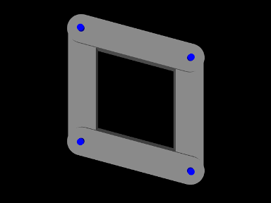
To model a four-bar in ArtiSynth presently requires adding compliance to the hinge joints. An example of this is defined by the demo program
artisynth.demos.tutorial.FourBarLinkage
shown in Figure 3.13. The code for the build() method and a couple of supporting methods is given below:
Two helper methods are used to construct the model: createLink()
(lines 6-17), and createJoint() (lines 23-36). createLink() makes the individual rigid bodies used to build the
linkage: a mesh is produced defining the body’s shape (a box with
rounded ends), and then passed to the
RigidBody
createFromMesh() method which creates the body and sets its
inertia according to a specified density. The body’s pose is then set
so as to center it at ![]() while rotating it about the
while rotating it about the ![]() axis
by the angle deg (in degrees). The completed body is then added to the
MechModel mech and returned.
axis
by the angle deg (in degrees). The completed body is then added to the
MechModel mech and returned.
The second helper method, createJoint(), connects two rigid
bodies (link0 and link1) together using a HingeJoint. Because we know the location of the joint in
body-relative coordinates, it is easier to create the joint using the
transforms ![]() and
and ![]() instead of
instead of ![]() :
: ![]() locates the joint at the top end of link0, at
locates the joint at the top end of link0, at ![]() ,
with the
,
with the ![]() axis parallel to the body’s
axis parallel to the body’s ![]() axis, while
axis, while ![]() similarly locates the joint at the bottom of link1. After the
joint is created and added to the MechModel, its render
properties are set so that its axis is drawn as a blue cylinder.
similarly locates the joint at the bottom of link1. After the
joint is created and added to the MechModel, its render
properties are set so that its axis is drawn as a blue cylinder.
The build() method itself begins by creating a MechModel
and setting damping parameters for the rigid bodies (lines
40-43). Next, createLink() is used to create and store the four
links (lines 46-50), and the left bar is attached to ground by making
it non-dynamic (line 52). The links are then connected together using
joints created by createJoint() (lines 55-59). Finally, uniform
compliance and damping values are set for each of the joint’s
bilateral constraints, using the setCompliance() and setDamping() methods (lines 63-72). Values are set for the first five
constraints, since for a HingeJoint these are the bilateral
constraints. The compliance value of ![]() was found
experimentally to be low enough so as to not cause noticeable
deflections in the joints. Given
was found
experimentally to be low enough so as to not cause noticeable
deflections in the joints. Given ![]() and an
average mass of around
and an
average mass of around ![]() for each link pair,
(3.18) suggests the damping factor of
for each link pair,
(3.18) suggests the damping factor of ![]() . Note that for this example, very similar settings could be
achieved by simply calling
. Note that for this example, very similar settings could be
achieved by simply calling
In principle, we only need to set compliance for the constraints that are redundant, but it can sometimes be difficult to determine exactly which these are. Also, different values are often needed for linear and rotary constraints; that is not necessary here because the links have unit length and so the linear and rotary units have similar scales.
3.4.11 Rendering joints
Most joints provide a means to render themselves in order to provide a graphical representation of their position and configuration. Control over this is achieved by setting various properties in the joint component, including both specialized properties and the standard render properties (Section 4.3) used by all renderable components.
All joints which are subclasses of JointBase support rendering of both their C and D coordinate frames, through the properties drawFrameC, drawFrameD, and axisLength. The first two properties are of the type Renderer.AxisDrawStyle (described in detail in Section 3.2.8), and can be set to LINE or ARROW to enable the coordinate axes to be drawn either as lines or solid arrows. The axisLength property has type double and specifies the length with which the axes are drawn. As with all properties, these properties can be set either in the GUI, or in code using accessor methods supplied by the joint:
Another pair of properties used by several joints is shaftLength and shaftRadius, which specify the length and radius used to draw shaft or axis structures associated with the joint. These are rendered as solid cylinders, using the color indicated by the faceColor rendering property. The default value of both properties is 0; if shaftLength is 0, then the structures are not drawn, while if shaftRadius is 0, a default value proportional to shaftLength is used. For example, to enable rendering of a blue shaft along the rotation axis of a hinge joint, one may use the code fragment
As another example, to enable rendering of a green ball about the center of a spherical joint, one may use the fragment
Specific joints may define additional properties to control how they are rendered.
![[LOGO]](data:image/png;base64,iVBORw0KGgoAAAANSUhEUgAAAAsAAAAOCAYAAAD5YeaVAAAAAXNSR0IArs4c6QAAAAZiS0dEAP8A/wD/oL2nkwAAAAlwSFlzAAALEwAACxMBAJqcGAAAAAd0SU1FB9wKExQZLWTEaOUAAAAddEVYdENvbW1lbnQAQ3JlYXRlZCB3aXRoIFRoZSBHSU1Q72QlbgAAAdpJREFUKM9tkL+L2nAARz9fPZNCKFapUn8kyI0e4iRHSR1Kb8ng0lJw6FYHFwv2LwhOpcWxTjeUunYqOmqd6hEoRDhtDWdA8ApRYsSUCDHNt5ul13vz4w0vWCgUnnEc975arX6ORqN3VqtVZbfbTQC4uEHANM3jSqXymFI6yWazP2KxWAXAL9zCUa1Wy2tXVxheKA9YNoR8Pt+aTqe4FVVVvz05O6MBhqUIBGk8Hn8HAOVy+T+XLJfLS4ZhTiRJgqIoVBRFIoric47jPnmeB1mW/9rr9ZpSSn3Lsmir1fJZlqWlUonKsvwWwD8ymc/nXwVBeLjf7xEKhdBut9Hr9WgmkyGEkJwsy5eHG5vN5g0AKIoCAEgkEkin0wQAfN9/cXPdheu6P33fBwB4ngcAcByHJpPJl+fn54mD3Gg0NrquXxeLRQAAwzAYj8cwTZPwPH9/sVg8PXweDAauqqr2cDjEer1GJBLBZDJBs9mE4zjwfZ85lAGg2+06hmGgXq+j3+/DsixYlgVN03a9Xu8jgCNCyIegIAgx13Vfd7vdu+FweG8YRkjXdWy329+dTgeSJD3ieZ7RNO0VAXAPwDEAO5VKndi2fWrb9jWl9Esul6PZbDY9Go1OZ7PZ9z/lyuD3OozU2wAAAABJRU5ErkJggg==)