4.9 Custom Joints
If desired, it is also possible for applications to create their own custom joints. This involves creating two custom classes: a coupling class that does the constraint computations, and a joint class that wraps around it and allows it to connect connectable bodies. Details on how to create these classes are given in Sections 4.9.3 and 4.9.4, after some explanation of the constraint mechanism that underlies joint operation.
This section assumes that the reader is highly familiar with spatial kinematics and dynamics.
4.9.1 Joint constraints
To create a custom joint, it is necessary to understand how joints are
implemented. The basic function of a joint is to constrain the set of
poses allowed by the joint transform ![]() that relates frame C to
D. To do this, the joint imposes restrictions on the six-dimensional
spatial velocity
that relates frame C to
D. To do this, the joint imposes restrictions on the six-dimensional
spatial velocity ![]() that describes how frame C is moving
with respect to D. This restriction is done using a set of bilateral
constraints
that describes how frame C is moving
with respect to D. This restriction is done using a set of bilateral
constraints ![]() and (in some cases) unilateral constraints
and (in some cases) unilateral constraints ![]() ,
each of which is a
,
each of which is a ![]() matrix that acts to restrict a single
degree of freedom in
matrix that acts to restrict a single
degree of freedom in ![]() (see Section
A.5 for a review of
spatial velocities and forces). Bilateral constraints take the form of
an equality,
(see Section
A.5 for a review of
spatial velocities and forces). Bilateral constraints take the form of
an equality,
| (4.22) |
while unilateral constraints take the form of an inequality:
| (4.23) |
These constraints are defined with respect to frame C, and their total
number equals the number of DOFs that the joint removes. A
joint’s main computational task is to specify these
constraints. ArtiSynth then uses its own knowledge of how frames C and
D are connected to bodies A and B (or ground, if there is no body B)
to map the individual ![]() and
and ![]() onto the joint’s full
bilateral and unilateral constraint matrices
onto the joint’s full
bilateral and unilateral constraint matrices ![]() and
and ![]() (see
(3.4) and (3.5)) that restrict the
body velocities.
(see
(3.4) and (3.5)) that restrict the
body velocities.
As a simple example, consider a cylindrical joint, in which C is free
to rotate about and translate along the ![]() axis of D but other
motions are restricted. Letting
axis of D but other
motions are restricted. Letting ![]() and
and ![]() denote the
translational and rotational components of
denote the
translational and rotational components of ![]() , such that
, such that
we see that the constraints must enforce
| (4.24) |
This can be accomplished using four constraints defined as follows:
Constraining velocities is a necessary but insufficient condition for
constraint enforcement. Because of numerical errors, as well as the
fact that constraints are often nonlinear, the joint transform
![]() will tend to drift away from the joint restrictions as the
simulation proceeds, leading to the error
will tend to drift away from the joint restrictions as the
simulation proceeds, leading to the error ![]() described at the
end of Section 3.4.1. These errors are corrected
during a position correction at the end of every simulation time
step: the joint first projects
described at the
end of Section 3.4.1. These errors are corrected
during a position correction at the end of every simulation time
step: the joint first projects ![]() onto the nearest valid
constraint surface to form
onto the nearest valid
constraint surface to form ![]() , and
, and ![]() is then computed from
is then computed from
| (4.25) |
Because ![]() is (usually) small, we can approximate it as
a twist
is (usually) small, we can approximate it as
a twist ![]() representing a small displacement from frame
G (which lies on the constraint surface) to frame C. During the
position correction, ArtiSynth adjusts the pose of C relative to D in
order to try and bring
representing a small displacement from frame
G (which lies on the constraint surface) to frame C. During the
position correction, ArtiSynth adjusts the pose of C relative to D in
order to try and bring ![]() to zero. To do this, it uses
an estimate of the distance
to zero. To do this, it uses
an estimate of the distance ![]() along each constraint to the
constraint surface, which it computes from the dot product of
along each constraint to the
constraint surface, which it computes from the dot product of ![]() and
and ![]() :
:
| (4.26) |
ArtiSynth assembles these distances into a composite distance vector
![]() for all bilateral constraints, and then uses the system
solver to find a displacement
for all bilateral constraints, and then uses the system
solver to find a displacement ![]() of the system coordinates
that satisfies
of the system coordinates
that satisfies
Adding ![]() to the system coordinates
to the system coordinates ![]() then reduces the
constraint errors. While for nonlinear constraints several steps may be
required to bring the error to 0, the process usually converges
quickly.
then reduces the
constraint errors. While for nonlinear constraints several steps may be
required to bring the error to 0, the process usually converges
quickly.
Unlike bilateral constraints, unilateral constraints are one-sided,
and take effect, or are engaged, only when ![]() encounters
an inadmissible region. The constraint then acts to prevent further
penetration into the region, via the velocity restriction
(4.23), and also to push
encounters
an inadmissible region. The constraint then acts to prevent further
penetration into the region, via the velocity restriction
(4.23), and also to push ![]() out of the
inadmissible region, using a position correction analogous to that
used for bilateral constraints.
out of the
inadmissible region, using a position correction analogous to that
used for bilateral constraints.
Whether or not a unilateral constraint is engaged is determined by its
engaged value ![]() , which takes one of the three values:
, which takes one of the three values:
![]() , and is updated by the joint implementation as the
simulation proceeds. A value of 0 means that the constraint is not
engaged, and will not be included in the joint’s unilateral
constraint matrix
, and is updated by the joint implementation as the
simulation proceeds. A value of 0 means that the constraint is not
engaged, and will not be included in the joint’s unilateral
constraint matrix ![]() . Otherwise, if
. Otherwise, if ![]() is
is ![]() or
or ![]() , then the
constraint is engaged and will be included in
, then the
constraint is engaged and will be included in ![]() , using
, using ![]() if
if
![]() , or its negative
, or its negative ![]() if
if ![]() .
. ![]() therefore
defines a sign for the constraint. General details on how
unilateral constraints should be engaged or disengaged are discussed
in Section 4.9.2.
therefore
defines a sign for the constraint. General details on how
unilateral constraints should be engaged or disengaged are discussed
in Section 4.9.2.
A common use of unilateral constraints is to implement limits on joint
coordinate values; this also illustrates the utility of ![]() . For
example, the cylindrical joint mentioned above may have two
coordinates,
. For
example, the cylindrical joint mentioned above may have two
coordinates, ![]() and
and ![]() , describing the translation and rotation
along and about the D frame’s
, describing the translation and rotation
along and about the D frame’s ![]() axis. Now suppose we wish to bound
axis. Now suppose we wish to bound
![]() , such that
, such that
| (4.27) |
When these limits are violated, a unilateral constraint can be engaged
to limit motion along the ![]() axis.
A constraint
axis.
A constraint ![]() that will do this is
that will do this is
Whenever ![]() , using
, using ![]() in (4.23)
will ensure that
in (4.23)
will ensure that ![]() and hence
and hence ![]() will not fall further
below the lower bound. On the other hand, when
will not fall further
below the lower bound. On the other hand, when ![]() ,
we want to employ
,
we want to employ ![]() in (4.23) to ensure that
in (4.23) to ensure that
![]() . In other words, lower bounds can be enforced by
engaging
. In other words, lower bounds can be enforced by
engaging ![]() with
with ![]() , while upper bounds can be enforced
with
, while upper bounds can be enforced
with ![]() .
.
As with bilateral constraints, constraining velocities is not
sufficient; it is also necessary to correct position errors,
particularly as unilateral constraints are typically not engaged until
the inadmissible region is violated. The position correction procedure
is the same: for each engaged unilateral constraint, find a distance
![]() along its constraint direction that indicates the distance to
the inadmissible region boundary. ArtiSynth will then assemble these
along its constraint direction that indicates the distance to
the inadmissible region boundary. ArtiSynth will then assemble these
![]() into a composite distance vector
into a composite distance vector ![]() for all unilateral
constraints, and solve for a system coordinate displacement
for all unilateral
constraints, and solve for a system coordinate displacement ![]() that satisfies
that satisfies
| (4.28) |
Because of the inequality direction in
(4.28), distances ![]() representing
penetration into an inadmissible region must be negative. For
coordinate bounds such as (4.27), we need to use
representing
penetration into an inadmissible region must be negative. For
coordinate bounds such as (4.27), we need to use ![]() for the lower bound and
for the lower bound and ![]() for
the upper bound. Alternatively, if the unilateral constraint has been
included into the projection of C onto G and hence into the error term
for
the upper bound. Alternatively, if the unilateral constraint has been
included into the projection of C onto G and hence into the error term
![]() ,
, ![]() can be computed from
can be computed from
| (4.29) |
Note that unilateral constraints for coordinate limits are not
usually incorporated into the ![]() projection; more details on this are
given in Section 4.9.4.
projection; more details on this are
given in Section 4.9.4.
As simulation proceeds, the velocity limits imposed by
(4.22) and (4.23) are enforced by
bilateral and unilateral
constraint forces ![]() and
and ![]() whose
magnitudes are given by
whose
magnitudes are given by
| (4.30) |
where ![]() and
and ![]() are the Lagrange multipliers computed
by the mechanical system solver (and are components of
are the Lagrange multipliers computed
by the mechanical system solver (and are components of ![]() or
or
![]() in (1.10) and (1.13)).
in (1.10) and (1.13)).
![]() and
and ![]() are 6 DOF spatial force vectors, or wrenches
(Section A.5), which like
are 6 DOF spatial force vectors, or wrenches
(Section A.5), which like ![]() and
and
![]() are expressed in frame C. Because
are expressed in frame C. Because ![]() and
and ![]() are
proportional to spatial wrenches, they are often themselves referred
to as constraint wrenches, and within the ArtiSynth codebase are
described by a Wrench object.
are
proportional to spatial wrenches, they are often themselves referred
to as constraint wrenches, and within the ArtiSynth codebase are
described by a Wrench object.
4.9.2 Unilateral constraint engagement
As mentioned above, joints which implement unilateral constraints must
monitor ![]() and the joint coordinates as the simulation proceeds
and decide when to engage or disengage them.
and the joint coordinates as the simulation proceeds
and decide when to engage or disengage them.
Engagement is usually easy: a constraint is engaged whenever ![]() or a joint coordinate hits an inadmissible region. The constraint
or a joint coordinate hits an inadmissible region. The constraint
![]() is itself a spatial vector that is (locally) perpendicular to
the inadmissible region boundary, and
is itself a spatial vector that is (locally) perpendicular to
the inadmissible region boundary, and ![]() is chosen to be either
is chosen to be either
![]() or
or ![]() so that
so that ![]() is directed away from the
inadmissible region. In the remainder of this section, we shall assume
is directed away from the
inadmissible region. In the remainder of this section, we shall assume
![]() .
.
To disengage, we usually want to ensure that the joint configuration
is out of the inadmissible region. If we have a constraint ![]() ,
with a local distance
,
with a local distance ![]() defined such that
defined such that ![]() implies the
joint is inside the region, then we are out of the region when
implies the
joint is inside the region, then we are out of the region when
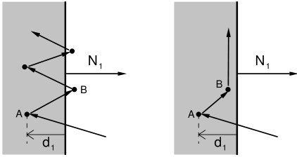
![]() . However, if we use only this as the disengagement
criterion, we may encounter a problem known as chattering,
illustrated in Figure 4.23 (left). An inadmissible
region is shown in gray, with a unilateral constraint
. However, if we use only this as the disengagement
criterion, we may encounter a problem known as chattering,
illustrated in Figure 4.23 (left). An inadmissible
region is shown in gray, with a unilateral constraint ![]() perpendicular to its boundary. As simulation proceeds, the joint lands
inside the region at an initial point A at the lower left, at a
(negative) distance
perpendicular to its boundary. As simulation proceeds, the joint lands
inside the region at an initial point A at the lower left, at a
(negative) distance ![]() from the boundary. Ideally the position
correction step will move the configuration by
from the boundary. Ideally the position
correction step will move the configuration by ![]() so that it lands
right on the region boundary. However, numerical errors and
nonlinearities may mean that in fact it lands outside the
region, at point B. Then on the next step it reenters the region, only
to again be pushed out, etc.
so that it lands
right on the region boundary. However, numerical errors and
nonlinearities may mean that in fact it lands outside the
region, at point B. Then on the next step it reenters the region, only
to again be pushed out, etc.
ArtiSynth implements two solutions to chattering. One is to implement
a deadband, so that instead of correcting the position by
![]() , we correct it by
, we correct it by ![]() , where
, where ![]() is a penetration tolerance. This means that the correction will
try to leave the joint inside the region by a small amount (Figure
4.23, right) so that chattering is suppressed. The
penetration tolerance used depends on the constraint type. Those that
are primarily linear use the value of the penetrationTol
property, while those that are primarily rotary use the value of the
rotaryLimitTol property; both of these are exported as
inheritable properties by both
MechModel and
BodyConnector, with default
values computed from the model’s overall dimensions.
is a penetration tolerance. This means that the correction will
try to leave the joint inside the region by a small amount (Figure
4.23, right) so that chattering is suppressed. The
penetration tolerance used depends on the constraint type. Those that
are primarily linear use the value of the penetrationTol
property, while those that are primarily rotary use the value of the
rotaryLimitTol property; both of these are exported as
inheritable properties by both
MechModel and
BodyConnector, with default
values computed from the model’s overall dimensions.
The second chattering solution is to disengage only when the joint is
actively moving away from the region, as determined by ![]() .
The disengagement criteria then become
.
The disengagement criteria then become
| (4.31) |
![]() is called the contact speed and can be computed from
is called the contact speed and can be computed from
| (4.32) |
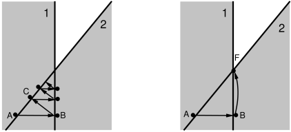
Another problem, which we call constraint oscillation, can occur when we are near two or more overlapping inadmissible regions whose boundaries are not perpendicular. See Figure 4.24 (left), which shows two overlapping regions 1 and 2. The joint starts at point A, inside region 1 but just outside region 2. Since only constraint 1 is engaged, the position correction moves it toward the boundary of 1, overshooting and landing at point B outside of 1 but inside region 2. Constraint 2 now engages, moving the joint to C, where it is past the boundary of 2 but inside 1 again. While the example in the figure converges to the corner where the boundaries of 1 and 2 meet, convergence may be slow and may be prevented entirely by external forcing. While the mechanisms that prevent chattering may also prevent oscillation, we find that an additional measure is useful, which is to simply require that a constraint must be engaged for at least two simulation steps. The result is shown in Figure 4.24 (right), where after the joint arrives at B, constraint 1 remains engaged along with constraint 2, and the subsequent solution takes the joint directly to point F at the corner where 1 and 2 meet.
4.9.3 Implementing a custom joint
All of the work of computing joint constraints and coordinates, as described in the previous sections, is done within a “coupling” class which is a subclass of RigidBodyCoupling. An instance of this is then embedded within a “joint” class (which is a subclass of JointBase) that supports connections with other bodies, provides rendering, exports various properties, and allows the joint to be attached to a MechModel.
For purposes of this discussion, we will assume that these two custom classes are called CustomCoupling and CustomJoint, respectively. The implementation of CustomJoint can be as simple as this:
This creates an instance of CustomCoupling and sets it to the (inherited) myCoupling attribute inside the default constructor (which is where this normally should be done). Another constructor is provided which uses setBodies() to create a joint that is attached to two bodies with the D frame specified in world coordinates. In practice, a joint may also export some properties (such as joint coordinates), provide additional constructors, and implement rendering; one should examine the source code for some existing joints.
4.9.4 Implementing a custom coupling
Implementing a custom coupling constitutes most of the effort in
creating a custom joint, since the coupling is responsible for
maintaining the constraints ![]() and
and ![]() that enforce the joint
behavior.
that enforce the joint
behavior.
Before proceeding, we discuss the coordinate frame in which these
constraints are situated. It is often convenient to describe joint
constraints with respect to frame C, since rotations are frequently
centered there. However, the joint transform ![]() usually
contains errors (Section 3.4.1) due to a
combination of simulation error and possible joint compliance. To
determine these errors, we project C onto another frame G, defined to
be the nearest to C that is consistent with the bilateral (and possibly
some unilateral) constraints. (This is done by the projectToConstraints() method, described below). The result is a
joint transform
usually
contains errors (Section 3.4.1) due to a
combination of simulation error and possible joint compliance. To
determine these errors, we project C onto another frame G, defined to
be the nearest to C that is consistent with the bilateral (and possibly
some unilateral) constraints. (This is done by the projectToConstraints() method, described below). The result is a
joint transform ![]() that is “error free” with respect to
bilateral constraints and also consistent with the coordinates (if
supported). This makes it convenient to formulate constraints with
respect to frame G instead of C, and so this is the convention
ArtiSynth uses. In particular, the updateConstraints() method,
described below, uses
that is “error free” with respect to
bilateral constraints and also consistent with the coordinates (if
supported). This makes it convenient to formulate constraints with
respect to frame G instead of C, and so this is the convention
ArtiSynth uses. In particular, the updateConstraints() method,
described below, uses ![]() , together with the spatial velocity
, together with the spatial velocity
![]() describing the motion of G with respect to D.
describing the motion of G with respect to D.
An actual custom coupling implementation involves subclassing RigidBodyCoupling and then implementing five abstract methods, the outline of which looks like this:
The implementations of these methods are now described in detail.
initializeConstraints()
This method has the signature
and is called in the coupling’s superclass constructor (i.e., the constructor for RigidBodyCoupling). It is responsible for initializing the coupling’s constraints and (if supported) coordinates.
Constraints are added using one of the two superclass methods:
Each creates a new RigidBodyConstraint and adds it to the coupling’s constraint list. flags is an or-ed combination of the following flags defined in RigidBodyConstraint:
- BILATERAL
-
Constraint is bilateral (i.e., an equality). If BILATERAL is not specified, the constraint is considered unilateral.
- ROTARY
-
Constraint primarily restricts rotary motion. If it is unilateral, the joint’s rotaryLimitTol property is used for its penetration tolerance.
- LINEAR
-
Constraint primarily restricts translational motion. If it is unilateral, the joint’s penetrationTol property is used for its penetration tolerance.
- CONSTANT
-
Constraint is constant with respect to frame G. This flag is set automatically if the constraint is created using addConstraint(flags,wrench).
- LIMIT
-
Constraint is used to enforce limits for a coordinate. This flag is set automatically if the constraint is specified as the limit constraint for a coordinate.
The method addConstraint(flags,wrench) takes an additional Wrench argument specifying the (presumed constant) value of the constraint with respect to frame G, and sets the CONSTANT flag just described.
Coordinates are added similarly using using one of the two superclass methods:
Each creates a new CoordinateInfo object (which is an inner class
of RigidBodyCoupling), and adds it to the
coupling’s coordinate list. In the second method, min and max give
the initial range limits, and limCon, if non-null, specifies a
constraint (previously created using addConstraint) that is parallel to
the twist associated with the coordinate’s motion and which can be used for
enforcing the limits. Specifying a non-null limCon will cause the
constraint’s LIMIT flag to be set. The argument flags is reserved
for future use and should be set to 0. If not specified, the default coordinate
limits are ![]() .
.
Each coordinate is associated with a twist value which describes the instantaneous spatial velocity imparted by that coordinate in frame G. The twist value for each coordinate must be specified by the coupling, using the method
where cidx is the coordinate index and twistG is the current value of the twist expressed in coordinate frame G. If the twist has a constant value, setCoordinateTwist() may be called once in initializeConstraints(). Otherwise, it must be called in updateConstraints().
The implementation of initializeConstraints() for a coupling that implements a hinge type joint might look like this:
Six constraints are specified, with the sixth being a unilateral constraint that enforces the limits on the single coordinate describing the rotation angle. Each constraint and coordinate has an integer index giving the location in its list, in the order it was added. This index can be used to later retrieve the RigidBodyConstraint or CoordinateInfo object for the constraint or coordinate, using the methods getConstraint(idx) or getCoordinateInfo(idx).
Because initializeConstraints() is called in the superclass constructor, member attributes for the custom coupling will not yet be initialized when it is first called. Therefore, the method should not depend on the initial values of non-static member variables. initializeConstraints() can also be called later to rebuild the constraints if some defining setting is changed.
coordinatesToTCD()
This method has the signature
and is called when needed by the system. If coordinates are supported,
then the transform ![]() should be set from the coordinate values
supplied in coords, and returned in the argument TCD.
Otherwise, this method should do nothing.
should be set from the coordinate values
supplied in coords, and returned in the argument TCD.
Otherwise, this method should do nothing.
TCDToCoordinates()
This method has the signature
and is called when needed by the system. It is the inverse of coordinatesToTCD(): if coordinates are supported, then their values
should be set from the joint transform ![]() supplied by TCD
and returned in coords. Otherwise, this method should do
nothing.
supplied by TCD
and returned in coords. Otherwise, this method should do
nothing.
When calling this method, it is assumed that TCD is “legal” with respect to the joint’s constraints (as defined by projectToConstraints(), described next). If this is not the case, then projectToConstraints() should be called instead.
One issue that can arise is when a coordinate represents an angle
![]() that has a range greater than
that has a range greater than ![]() . In that case, a common
strategy is to compute a nominal value for
. In that case, a common
strategy is to compute a nominal value for ![]() , and then add or
subtract
, and then add or
subtract ![]() from it until the resulting value is as close as
possible to the current value for the angular coordinate. This
allows the angle to wrap through its entire range. To implement this,
one can use the method
from it until the resulting value is as close as
possible to the current value for the angular coordinate. This
allows the angle to wrap through its entire range. To implement this,
one can use the method
in the coordinate’s CoordinateInfo object, which finds the angle equivalent to phi that is nearest to the current coordinate value.
Coordinate values computed by this method should not be clipped to their ranges.
projectToConstraints()
This method has the signature
and is called when needed by the system. It is responsible for
projecting the joint transform ![]() (supplied by TCD) onto
the nearest transform
(supplied by TCD) onto
the nearest transform ![]() that is valid for the bilateral
constraints, and returning this in TGD. If coordinates are
supported and coords is non-null, then the coordinate
values corresponding to
that is valid for the bilateral
constraints, and returning this in TGD. If coordinates are
supported and coords is non-null, then the coordinate
values corresponding to ![]() should also be computed and returned
in coords. The easiest way to do this is to simply call TCDToCoordinates(TGD,coords), although in some cases it may be
computationally cheaper to compute both the coordinates and the
projection at the same time.
should also be computed and returned
in coords. The easiest way to do this is to simply call TCDToCoordinates(TGD,coords), although in some cases it may be
computationally cheaper to compute both the coordinates and the
projection at the same time.
Optionally, the coupling may also extend the projection to include
unilateral constraints that are not associated with coordinate
limits. In particular, this should be done for constraints for which
it is desired to have the constraint error included in ![]() and
the corresponding argument errC that is passed to updateConstraints().
and
the corresponding argument errC that is passed to updateConstraints().
updateConstraints()
This method has the signature
and is usually called once per simulation time step. It is responsible for:
-
•
Updating the values of all non-constant constraint wrenches, including the limit constraints for joint coordinates, along with their derivatives.
-
•
Updating the coordinate twists for couplings with joint coordinates, using the method setCoordinateTwist() described above. (For twists that are constant, setCoordinateTwist() can be called in initializeConstraints() instead.)
-
•
If updateEngaged is true, updating the engaged and distance attributes for all unilateral constraints not associated with a coordinate limit.
The method supplies several arguments:
-
•
TGD, containing the idealized joint transform
 from frame G to D produced by calling projectToConstraints().
-
•
TCD, containing the joint transform
 from
frame C to D and supplied for legacy reasons.
from
frame C to D and supplied for legacy reasons. -
•
errC, representing the (hopefully small) error transform
 from frame C to G as a spatial twist vector.
 -
•
velGD, giving the spatial velocity
 of frame
G with respect to D, as seen in G; this is needed to compute wrench
derivatives.
of frame
G with respect to D, as seen in G; this is needed to compute wrench
derivatives. -
•
updateEngaged, which requests the updating of unilateral engaged and distance attributes as described above.
If the coupling supports coordinates, their values will be updated
before the method is called so as to correspond to ![]() . If
needed, a coordinate’s value may be obtained from the value
attribute of its CoordinateInfo object, which may in turn be
obtained using getCoordinateInfo(idx). Likewise, RigidBodyConstraint objects for each constraint may be obtained using
getConstraint(idx).
. If
needed, a coordinate’s value may be obtained from the value
attribute of its CoordinateInfo object, which may in turn be
obtained using getCoordinateInfo(idx). Likewise, RigidBodyConstraint objects for each constraint may be obtained using
getConstraint(idx).
Constraint wrenches correspond to ![]() and
and ![]() in Section
4.9.1. These, along with their derivatives
in Section
4.9.1. These, along with their derivatives
![]() and
and ![]() , are described by the wrenchG and dotWrenchG attributes of each constraint’s
RigidBodyConstraint object, and may
be managed by a variety of methods:
, are described by the wrenchG and dotWrenchG attributes of each constraint’s
RigidBodyConstraint object, and may
be managed by a variety of methods:
dotWrenchG is used in computing the constraint offset terms
and
that appear in (3.3) and (1.13). While these improve the computational accuracy of the simulation, their effect is often small, and so in practice one may be able to omit computing dotWrenchG and instead leave its value as 0.
Wrench information must also be computed for unilateral constraints
which implement coordinate limits. While it is not necessary to
compute the distance and engaged attributes for these
constraints (this is done automatically), it is necessary to
ensure that the wrench’s magnitude is compatible with the coordinate’s
speed. More precisely, if the coordinate is given by ![]() , then the
limit wrench
, then the
limit wrench ![]() must have a magnitude such that
must have a magnitude such that
| (4.33) |
As mentioned above, if updateEngaged is true, the engaged and distance attributes for unilateral constraints not
associated with coordinate limits must be updated. These correspond
to ![]() and
and ![]() in Section 4.9.1, and are
contained in the constraint’s
RigidBodyConstraint object and may
be queried using the methods
in Section 4.9.1, and are
contained in the constraint’s
RigidBodyConstraint object and may
be queried using the methods
It is up to updateConstraints() to compute the distance, with
a negative value denoting penetration into the inadmissible
region. If projectToConstraints() is
implemented so as to account for the constraint, then ![]() will
be projected out of the inadmissible region and the distance will be
implicitly present in
will
be projected out of the inadmissible region and the distance will be
implicitly present in ![]() and so can be recovered by taking
the dot product of the constraint wrench and velGD:
and so can be recovered by taking
the dot product of the constraint wrench and velGD:
Otherwise, if the constraint is not accounted for in projectToConstraints(), the distance must be obtained by other means.
To update engaged, one may use the general convenience method
which sets engaged according to the rules of Section 4.9.2, for an inadmissible region corresponding to dist < dmin or dist > dmax. The upper or lower bounds may be removed by setting dmin to -inf or dmax to inf, respectively.
4.9.5 Example: a simple custom joint
 |
 |
A simple model illustrating custom joint creation is provided by
artisynth.demos.tutorial.CustomJointDemo
This implements a joint class defined by CustomJoint (also in the package artisynth.demos.tutorial), which is actually just a simple implementation of SlottedHingeJoint (Section 3.5.4). Certain details are omitted, such as exporting coordinate values and ranges as properties, and other things are simplified, such as the rendering code. One may consult the source code for SlottedHingeJoint to obtain a more complete example.
This section will focus on the implementation of the joint coupling, which is created as an inner class of CustomJoint called CustomCoupling and which (like all couplings) extends RigidBodyCoupling. The joint itself creates an instance of the coupling in its default constructor, exactly as described in Section 4.9.3.
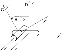
The coupling allows two DOFs (Figure 4.25, left):
translation along the ![]() axis of D (described by the coordinate
axis of D (described by the coordinate ![]() ),
and rotation about the
),
and rotation about the ![]() axis of D (described by the coordinate
axis of D (described by the coordinate
![]() ), with
), with ![]() related to the coordinates by
(3.19). It implements
initializeConstraints() as follows:
related to the coordinates by
(3.19). It implements
initializeConstraints() as follows:
Six constraints are added using addConstraint(): two linear bilaterals to
restrict translation along the ![]() and
and ![]() axes of D, two rotary bilaterals to
restrict rotation about the
axes of D, two rotary bilaterals to
restrict rotation about the ![]() and
and ![]() axes of D, and two unilaterals to
enforce limits on
axes of D, and two unilaterals to
enforce limits on ![]() and
and ![]() . Four of the constraints are constant in
frame G, and so are initialized with a wrench value. The other two are not
constant in G and so will need to be updated in updateConstraints(). The
coordinates for
. Four of the constraints are constant in
frame G, and so are initialized with a wrench value. The other two are not
constant in G and so will need to be updated in updateConstraints(). The
coordinates for ![]() and
and ![]() are added at the end, using addCoordinate(), with default joint limits and a reference to the constraint
that will enforce the limit. The twist for
are added at the end, using addCoordinate(), with default joint limits and a reference to the constraint
that will enforce the limit. The twist for ![]() is constant and so it is
initialized here as well.
is constant and so it is
initialized here as well.
The implementations for coordinatesToTCD() and TCDToCoordinates() simply use (3.19) to
compute ![]() from the coordinates, or vice versa:
from the coordinates, or vice versa:
X_IDX and THETA_IDX are constants defining the
coordinate indices for ![]() and
and ![]() . In TCDToCoordinates(),
note the use of the CoordinateInfo method nearestAngle(), as discussed in Section
4.9.4.
. In TCDToCoordinates(),
note the use of the CoordinateInfo method nearestAngle(), as discussed in Section
4.9.4.
Projecting ![]() onto the error-free
onto the error-free ![]() is done by projectToConstraints(), implemented as follows:
is done by projectToConstraints(), implemented as follows:
The translational projection is easy - the y and z components of the
translation vector p are simply zeroed out. To project the
rotation R, we use its rotateZDirection() method, which
applies the shortest rotation aligning its ![]() axis with
axis with ![]() . The residual rotation will be a rotation in the
. The residual rotation will be a rotation in the ![]() -
-![]() plane.
If coords is non-null and needs to be computed, we simply
call TCDToCoordinates().
plane.
If coords is non-null and needs to be computed, we simply
call TCDToCoordinates().
Lastly, the implementation for updateConstraints() is as follows:
Only constraints 0 and 4 need to have their wrenches updated, since
the rest are constant, and we obtain their constraint objects using
getConstraint(idx). Constraint 0 restricts motion along the ![]() axis in D, and while this is constant in D, it is not constant
in G, which is where the wrench must be situated. The
axis in D, and while this is constant in D, it is not constant
in G, which is where the wrench must be situated. The ![]() axis of D
as seen in G is the given by the second row of the rotation matrix of
axis of D
as seen in G is the given by the second row of the rotation matrix of
![]() , which from (3.19) we see is
, which from (3.19) we see is
![]() , where
, where ![]() and
and
![]() . We obtain
. We obtain ![]() and
and ![]() directly from TGD, since this has been projected to lie on the constraint surface;
alternatively, we could compute them from
directly from TGD, since this has been projected to lie on the constraint surface;
alternatively, we could compute them from ![]() . To obtain the
wrench derivative, we note that
. To obtain the
wrench derivative, we note that ![]() and
and
![]() , and that
, and that ![]() is simply the
is simply the ![]() component of the angular velocity of
component of the angular velocity of ![]() with respect to
with respect to ![]() , or velGD.w.z. The wrench and its derivative are set using the
constraint’s setWrenchG() and setDotWrenchG() methods.
, or velGD.w.z. The wrench and its derivative are set using the
constraint’s setWrenchG() and setDotWrenchG() methods.
The other non-constant constraint is the limit constraint for the ![]() coordinate, which is the
coordinate, which is the ![]() axis of D as seen in G. This is updated
similarly. Since all unilateral constraints are coordinate limits, there is no
need to update their distance or engaged attributes as this is done
automatically by the system.
axis of D as seen in G. This is updated
similarly. Since all unilateral constraints are coordinate limits, there is no
need to update their distance or engaged attributes as this is done
automatically by the system.
Finally, we use setCoordinateTwist() to update the twist for the ![]() coordinate, which is the spatial velocity imparted by a change in
coordinate, which is the spatial velocity imparted by a change in ![]() as seen
in frame G. Although this twist has the constant value
as seen
in frame G. Although this twist has the constant value ![]() in
frame D, it varies in frame G according to the transform from
in
frame D, it varies in frame G according to the transform from ![]() to
to ![]() . In
this particular example, it has the same values as the
. In
this particular example, it has the same values as the ![]() limit constraint.
limit constraint.
![[LOGO]](data:image/png;base64,iVBORw0KGgoAAAANSUhEUgAAAAsAAAAOCAYAAAD5YeaVAAAAAXNSR0IArs4c6QAAAAZiS0dEAP8A/wD/oL2nkwAAAAlwSFlzAAALEwAACxMBAJqcGAAAAAd0SU1FB9wKExQZLWTEaOUAAAAddEVYdENvbW1lbnQAQ3JlYXRlZCB3aXRoIFRoZSBHSU1Q72QlbgAAAdpJREFUKM9tkL+L2nAARz9fPZNCKFapUn8kyI0e4iRHSR1Kb8ng0lJw6FYHFwv2LwhOpcWxTjeUunYqOmqd6hEoRDhtDWdA8ApRYsSUCDHNt5ul13vz4w0vWCgUnnEc975arX6ORqN3VqtVZbfbTQC4uEHANM3jSqXymFI6yWazP2KxWAXAL9zCUa1Wy2tXVxheKA9YNoR8Pt+aTqe4FVVVvz05O6MBhqUIBGk8Hn8HAOVy+T+XLJfLS4ZhTiRJgqIoVBRFIoric47jPnmeB1mW/9rr9ZpSSn3Lsmir1fJZlqWlUonKsvwWwD8ymc/nXwVBeLjf7xEKhdBut9Hr9WgmkyGEkJwsy5eHG5vN5g0AKIoCAEgkEkin0wQAfN9/cXPdheu6P33fBwB4ngcAcByHJpPJl+fn54mD3Gg0NrquXxeLRQAAwzAYj8cwTZPwPH9/sVg8PXweDAauqqr2cDjEer1GJBLBZDJBs9mE4zjwfZ85lAGg2+06hmGgXq+j3+/DsixYlgVN03a9Xu8jgCNCyIegIAgx13Vfd7vdu+FweG8YRkjXdWy329+dTgeSJD3ieZ7RNO0VAXAPwDEAO5VKndi2fWrb9jWl9Esul6PZbDY9Go1OZ7PZ9z/lyuD3OozU2wAAAABJRU5ErkJggg==)