ArtiSynth Modeling Guide
Last update: Apr 10, 2017
Contents:
- 1 ArtiSynth Overview
- 2 Supporting classes
- 3 Mechanical Models I
- 4 Mechanical Models II
- 5 Simulation Control
- 6 Finite Element Models
- 7 DICOM Images
- A Mathematical Review
Preface
This guide describes how to create mechanical and biomechanical models in ArtiSynth using its Java API.
It is assumed that the reader is familiar with basic Java programming, including variable assignment, control flow, exceptions, functions and methods, object construction, inheritance, and method overloading. Some familiarity with the basic I/O classes defined in java.io.*, including input and output streams and the specification of file paths using File, as well as the collection classes ArrayList and LinkedList defined in java.util.*, is also assumed.
How to read this guide
Section 1 offers a general overview of ArtiSynth’s software design, and briefly describes the algorithms used for physical simulation (Section 1.2). The latter section may be skipped on first reading. A more comprehensive overview paper is available online.
The remainder of the manual gives details instructions on how to build various types of mechanical and biomechanical models. Sections 3 and 4 give detailed information about building general mechanical models, involving particles, springs, rigid bodies, joints, constraints, and contact. Section 5 describes how to add control panels, controllers, and input and output data streams to a simulation. Section 6 describes how to incorporate finite element models. The required mathematics is reviewed in Section A.
If time permits, the reader will profit from a top-to-bottom read. However, this may not always be necessary. Many of the sections contain detailed examples, all of which are available in the package artisynth.demos.tutorial and which may be run from ArtiSynth using Models > All demos > tutorials. More experienced readers may wish to find an appropriate example and then work backwards into the text and preceeding sections for any needed explanatory detail.
Chapter 1 ArtiSynth Overview
ArtiSynth is an open-source, Java-based system for creating and simulating mechanical and biomechanical models, with specific capabilities for the combined simulation of rigid and deformable bodies, together with contact and constraints. It is presently directed at application domains in biomechanics, medicine, physiology, and dentistry, but it can also be applied to other areas such as traditional mechanical simulation, ergonomic design, and graphical and visual effects.
1.1 System structure
An ArtiSynth model is composed of a hierarchy of models and model components which are implemented by various Java classes. These may include sub-models (including finite element models), particles, rigid bodies, springs, connectors, and constraints. The component hierarchy may be in turn connected to various agent components, such as control panels, controllers and monitors, and input and output data streams (i.e., probes), which have the ability to control and record the simulation as it advances in time. Agents are presented in more detail in Section 5.
The models and agents are collected together within a top-level component known as a root model. Simulation proceeds under the control of a scheduler, which advances the models through time using a physics simulator. A rich graphical user interface (GUI) allows users to view and edit the model hierarchy, modify component properties, and edit and temporally arrange the input and output probes using a timeline display.
1.1.1 Model components
Every ArtiSynth component is an instance of ModelComponent. When connected to the hierarchy, it is assigned a unique number relative to its parent; the parent and number can be obtained using the methods getParent() and getNumber(), respectively. Components may also be assigned a name (using setName()) which is then returned using getName().
A sub-interface of ModelComponent includes CompositeComponent, which contains child components. A ComponentList is a CompositeComponent which simply contains a list of other components (such as particles, rigid bodies, sub-models, etc.).
Components which contain state information (such as position and velocity) should extend HasState, which provides the methods getState() and setState() for saving and restoring state.
A Model is a sub-interface of CompositeComponent and HasState that contains the notion of advancing through time and which implements this with the methods initialize(t0) and advance(t0, t1, flags), as discussed further in Section 1.1.4. The most common instance of Model used in ArtiSynth is MechModel (Section 1.1.5), which is the top-level container for a mechanical or biomechanical model.
1.1.2 The RootModel
The top-level component in the hierarchy is the root model, which is a subclass of RootModel and which contains a list of models along with lists of agents used to control and interact with these models. The component lists in RootModel include:
Each agent may be associated with a specific top-level model.
1.1.3 Component path names
The names and/or numbers of a component and its ancestors can be used to form a component path name. This path has a construction analogous to Unix file path names, with the ’/’ character acting as a separator. Absolute paths start with ’/’, which indicates the root model. Relative paths omit the leading ’/’ and can begin lower down in the hierarchy. A typical path name might be
/models/JawHyoidModel/axialSprings/lad
For nameless components in the path, their numbers can be used instead. Numbers can also be used for components that have names. Hence the path above could also be represented using only numbers, as in
/0/0/1/5
although this would most likely appear only in machine-generated output.
1.1.4 Model advancement
ArtiSynth simulation proceeds by advancing all of the root model’s top-level models through a sequence of time steps. Every time step is achieved by calling each model’s advance() method:
This method advances the model from time t0 to time t1, performing whatever physical simulation is required (see Section 1.2). The method may optionally return a StepAdjusment indicating that the step size (t1 - t0) was too large and that the advance should be redone with a smaller step size.
The root model has it’s own advance(), which in turn calls the advance method for all of the top-level models, in sequence. The advance of each model is surrounded by the application of whatever agents are associated with that model. This is done by calling the agent’s apply() method:
Agents not associated with a specific model are applied before (or after) the advance of all other models.
More precise details about model advancement are given in the ArtiSynth Reference Manual.
1.1.5 MechModel
Most ArtiSynth applications contain a single top-level model which is an instance of MechModel. This is a CompositeComponent that may (recursively) contain an arbitrary number of mechanical components, including finite element models, other MechModels, particles, rigid bodies, constraints, attachments, and various force effectors. The MechModel advance() method invokes a physics simulator that advances these components forward in time (Section 1.2).
For convenience each MechModel contains a number of predefined containers for different component types, including:
Each of these is a child component of MechModel and is implemented as a ComponentList. Special methods are provided for adding and removing items from them. However, applications are not required to use these containers, and may instead create any component containment structure that is appropriate. If not used, the containers will simply remain empty.
1.2 Physics simulation
Only a brief summary of ArtiSynth physics simulation is described here. Full details are given in [5] and in the related overview paper.
For purposes of physics simulation, the components of a MechModel are grouped as follows:
- Dynamic components
-
Components, such as a particles and rigid bodies, that contain position and velocity state, as well as mass. All dynamic components are instances of the Java interface DynamicComponent. - Force effectors
-
Components, such as springs or finite elements, that exert forces between dynamic components. All force effectors are instances of the Java interface ForceEffector. - Constrainers
-
Components that enforce constraints between dynamic components. All constrainers are instances of the Java interface Constrainer. - Attachments
-
Attachments between dynamic components. While technically these are constraints, they are implemented using a different approach. All attachment components are instances of DynamicAttachment.
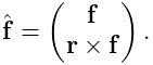
The positions, velocities, and forces associated with all the
dynamic components are denoted by the composite vectors
![]() ,
, ![]() , and
, and ![]() .
In addition, the composite mass matrix is given by
.
In addition, the composite mass matrix is given by
![]() .
Newton’s second law then gives
.
Newton’s second law then gives
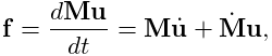 |
(1.1) |
where the ![]() accounts for various ``fictitious'' forces.
accounts for various ``fictitious'' forces.
Each integration step involves solving for
the velocities ![]() at time step
at time step ![]() given the velocities and forces
at step
given the velocities and forces
at step ![]() . One way to do this is to solve the expression
. One way to do this is to solve the expression
| (1.2) |
for ![]() , where
, where ![]() is the step size and
is the step size and
![]() . Given the updated velocities
. Given the updated velocities ![]() , one can
determine
, one can
determine ![]() from
from
| (1.3) |
where ![]() accounts for situations (like rigid bodies) where
accounts for situations (like rigid bodies) where ![]() , and then solve for the updated positions using
, and then solve for the updated positions using
| (1.4) |
(1.2) and (1.4) together comprise a simple symplectic Euler integrator.
In addition to forces, bilateral and unilateral constraints give rise to
locally linear constraints on ![]() of the form
of the form
| (1.5) |
Bilateral constraints may include rigid body joints, FEM
incompressibility, and point-surface constraints, while unilateral
constraints include contact and joint limits. Constraints give rise
to constraint forces (in the directions ![]() and
and ![]() )
which supplement the forces of (1.1) in order to enforce
the constraint conditions. In addition, for unilateral constraints,
we have a complementarity condition in which
)
which supplement the forces of (1.1) in order to enforce
the constraint conditions. In addition, for unilateral constraints,
we have a complementarity condition in which ![]() implies no
constraint force, and a constraint force implies
implies no
constraint force, and a constraint force implies ![]() . Any
given constraint usually involves only a few dynamic components and so
. Any
given constraint usually involves only a few dynamic components and so
![]() and
and ![]() are generally sparse.
are generally sparse.
Adding constraints to the velocity solve (1.2) leads to a mixed linear complementarity problem (MLCP) of the form
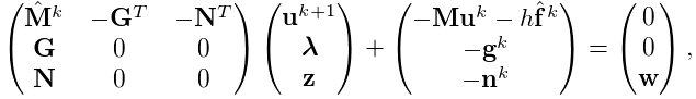 |
|||
| (1.6) |
where ![]() is a slack variable,
is a slack variable, ![]() and
and ![]() give the force
constraint impulses over the time step, and
give the force
constraint impulses over the time step, and ![]() and
and ![]() are derivative
terms arising if
are derivative
terms arising if ![]() and
and ![]() are time varying. In addition,
are time varying. In addition,
![]() and
and ![]() are
are ![]() and
and ![]() augmented with stiffness
and damping terms terms to accommodate implicit integration, which
is often required for problems involving deformable bodies.
augmented with stiffness
and damping terms terms to accommodate implicit integration, which
is often required for problems involving deformable bodies.
Attachments can be implemented by constraining the velocities of the attached components using special constraints of the form
| (1.7) |
where ![]() and
and ![]() denote the velocities of the attached and
non-attached components. The constraint matrix
denote the velocities of the attached and
non-attached components. The constraint matrix ![]() is
sparse, with a non-zero block entry for each master component to
which the attached component is connected. The simplest case involves
attaching a point
is
sparse, with a non-zero block entry for each master component to
which the attached component is connected. The simplest case involves
attaching a point ![]() to another point
to another point ![]() , with the simple velocity relationship
, with the simple velocity relationship
| (1.8) |
That means that ![]() has a single entry of
has a single entry of ![]() (where
(where ![]() is the
is the ![]() identity matrix) in the
identity matrix) in the ![]() -th block column.
Another common case involves connecting a point
-th block column.
Another common case involves connecting a point ![]() to
a rigid frame
to
a rigid frame ![]() . The velocity relationship for this is
. The velocity relationship for this is
| (1.9) |
where ![]() and
and ![]() are the translational and rotational
velocity of the frame and
are the translational and rotational
velocity of the frame and ![]() is the location of the point relative
to the frame’s origin (as seen in world coordinates). The corresponding
is the location of the point relative
to the frame’s origin (as seen in world coordinates). The corresponding
![]() contains a single
contains a single ![]() block entry of the form
block entry of the form
| (1.10) |
in the ![]() block column, where
block column, where
![[l]\equiv\left(\begin{matrix}0&-l_{z}&l_{y}\\
l_{z}&0&-l_{x}\\
-l_{y}&l_{x}&0\end{matrix}\right)](mi/mi17.png) |
(1.11) |
is a skew-symmetric cross product matrix.
The attachment constraints ![]() could be added directly to
(1.6), but their special form allows us to
explicitly solve for
could be added directly to
(1.6), but their special form allows us to
explicitly solve for ![]() , and hence reduce the size of
(1.6), by factoring out the attached velocities
before solution.
, and hence reduce the size of
(1.6), by factoring out the attached velocities
before solution.
The MLCP (1.6) corresponds to a single step integrator. However, higher order integrators, such as Newmark methods, usually give rise to MLCPs with an equivalent form. Most ArtiSynth integrators use some variation of (1.6) to determine the system velocity at each time step.
To set up (1.6), the MechModel component
hierarchy is traversed and the methods of the different component
types are queried for the required values. Dynamic components (type
DynamicComponent) provide ![]() ,
, ![]() , and
, and ![]() ; force effectors
(ForceEffector) determine
; force effectors
(ForceEffector) determine ![]() and the stiffness/damping
augmentation used to produce
and the stiffness/damping
augmentation used to produce ![]() ; constrainers (Constrainer) supply
; constrainers (Constrainer) supply ![]() ,
, ![]() ,
, ![]() and
and ![]() , and attachments (DynamicAttachment) provide the information needed to factor out
attached velocities.
, and attachments (DynamicAttachment) provide the information needed to factor out
attached velocities.
1.3 Basic packages
The core code of the ArtiSynth project is divided into three main packages, each with a number of sub-packages.
1.3.1 maspack
The packages under maspack contain general computational utilities that are independent of ArtiSynth and could be used in a variety of other contexts. The main packages are:
1.3.2 artisynth.core
The packages under artisynth.core contain the core code for ArtiSynth model components and its GUI infrastructure.
1.3.3 artisynth.demos
These packages contain demonstration models that illustrate ArtiSynth’s modeling capabilities:
1.4 Properties
ArtiSynth components expose properties, which provide a uniform interface for accessing their internal parameters and state. Properties vary from component to component; those for RigidBody include position, orientation, mass, and density, while those for AxialSpring include restLength and material. Properties are particularly useful for automatically creating control panels and probes, as described in Section 5. They are also used for automating component serialization.
Properties are described only briefly in this section; more detailed descriptions are available in the Maspack Reference Manual and the overview paper.
The set of properties defined for a component is fixed for that component’s class; while property values may vary between component instances, their definitions are class-specific. Properties are exported by a class through code contained in the class definition, as described in Section 5.2.
1.4.1 Property handles and paths
Each property has a unique name which may be used to obtain a property handle through which the property’s value may be queried or set for a particular component. Property handles are implemented by the class Property and are returned by the component’s getProperty() method. getProperty() takes a property’s name and returns the corresponding handle. For example, components of type Muscle have a property excitation, for which a handle may be obtained using a code fragment such as
Property handles can also be obtained for sub-components, using a property path that consists of a path to the sub-component followed by a colon ‘:’ and the property name. For example, to obtain the excitation property for a sub-component located by axialSprings/lad relative to a MechModel, one could use a call of the form
1.4.2 Composite and inheritable properties
Composite properties are possible, in which a property value is a composite object that in turn has sub-properties. A good example of this is the RenderProps class, which is associated with the property renderProps for renderable objects and which itself can have a number of sub-properties such as visible, faceStyle, faceColor, lineStyle, lineColor, etc.
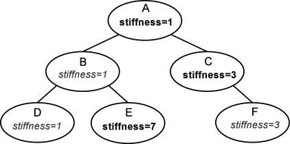
Properties can be declared to be inheritable, so that their values can be inherited from the same properties hosted by ancestor components further up the component hierarchy. Inheritable properties require a more elaborate declaration and are associated with a mode which may be either Explicit or Inherited. If a property’s mode is inherited, then its value is obtained from the closest ancestor exposing the same property whose mode is explicit. In Figure (1.1), the property stiffness is explicitly set in components A, C, and E, and inherited in B and D (which inherit from A) and F (which inherits from C).
1.5 Creating an application model
ArtiSynth applications are created by writing and compiling an application model that is a subclass of RootModel. This application-specific root model is then loaded and run by the ArtiSynth program.
The code for the application model should:
-
•
Declare a no-args constructor
-
•
Override the RootModel build() method to construct the application.
ArtiSynth can load a model either using the build method or by reading it from a file:
- Build method
-
ArtiSynth creates an instance of the model using the no-args constructor, assigns it a name (which is either user-specified or the simple name of the class), and then calls the build() method to perform the actual construction.
- Reading from a file
-
ArtiSynth creates an instance of the model using the no-args constructor, and then the model is named and constructed by reading the file.
The no-args constructor should perform whatever initialization is required in both cases, while the build() method takes the place of the file specification. Unless a model is originally created using a file specification (which is very tedious), the first time creation of a model will almost always entail using the build() method.
The general template for application model code looks like this:
Here, the model itself is called MyModel, and is defined in the (hypothetical) package artisynth.models.experimental (placing models in the super package artisynth.models is common practice but not necessary).
Note: The build() method was only introduced in ArtiSynth 3.1. Prior to that, application models were constructed using a constructor taking a String argument supplying the name of the model. This method of model construction still works but is deprecated.
1.5.1 Implementing the build() method
As mentioned above, the build() method is responsible for actual model construction. Many applications are built using a single top-level MechModel. Build methods for these may look like the following:
First, a MechModel is created (with the name "mech" in this example, although any name, or no name, may be given) and added to the list of models in the root model. Subsequent code then creates and adds the components required by the MechModel, as described in Sections 3, 4 and 6. The build() method also creates and adds to the root model any agents required by the application (controllers, probes, etc.), as described in Section 5.
When constructing a model, there is no fixed order in which components need to be added. For instance, in the above example, addModel(mech) could be called near the end of the build() method rather than at the beginning. The only restriction is that when a component is added to the hierarchy, all other components that it refers to should already have been added to the hierarchy. For instance, an axial spring (Section 3.1) refers to two points. When it is added to the hierarchy, those two points should already be present in the hierarchy.
The build() method supplies a String array as an argument, which can be used to transmit application arguments in a manner analogous to the args argument passed to static main() methods. In cases where the model is specified directly on the ArtiSynth command line (using the -model <classname> option), it is possible to also specify arguments for the build() method. This is done by enclosing the desired arguments within square brackets [ ] immediately following the -model option. So, for example,
> artisynth -model projects.MyModel [ -foo 123 ]
would cause the strings "-foo" and "123" to be passed to the build() method of MyModel.
1.5.2 Making models visible to ArtiSynth
In order to load an application model into ArtiSynth, the classes associated with its implementation must be made visible to ArtiSynth. This usually involves adding the top-level class directory associated with the application code to the classpath used by ArtiSynth.
The demonstration models referred to in this guide belong to the package artisynth.demos.tutorial and are already visible to ArtiSynth.
In most current ArtiSynth projects, classes are stored in a directory tree separate from the source code, with the top-level class directory named classes, located one level below the project root directory. A typical top-level class directory might be stored in a location like this:
/home/joeuser/artisynthProjects/classes
In the example shown in Section 1.5, the model was created in the package artisynth.models.experimental. Since Java classes are arranged in a directory structure that mirrors package names, with respect to the sample project directory shown above, the model class would be located in
/home/joeuser/artisynthProjects/classes/artisynth/models/experimental
At present there are three ways to make top-level class directories known to ArtiSynth:
- Add projects to your Eclipse launch configuration
-
If you are using the Eclipse IDE, then you can add the project in which are developing your model code to the launch configuration that you use to run ArtiSynth. Other IDEs will presumably provide similar functionality.
- Add the directories to the EXTCLASSPATH file
-
You can explicitly list class directories in the file EXTCLASSPATH, located in the ArtiSynth root directory (it may be necessary to create this file).
- Add the directories to your CLASSPATH environment variable
-
If you are running ArtiSynth from the command line, using the artisynth command (or artisynth.bat on Windows), then you can define a CLASSPATH environment variable in your environment and add the needed directories to this.
1.5.3 Loading and running a model
If a model’s classes are visible to ArtiSynth, then it may be loaded into ArtiSynth in several ways:
- Loading by class path
-
A model may be loaded by directly by choosing File > Load from class ... and directly specifying its class name. It is also possible to use the -model <classname> command line argument to have a model loaded directly into ArtiSynth when it starts up.
- Loading from the Models menu
-
A faster way to load a model is by selecting it in one of the Models submenus. This may require editing the model menu configuration files.
- Loading from a file
-
If a model has previously been saved to a file, it may be loaded from that file by choosing File > Load model ....
These methods are described in detail in the section ``Loading and Simulating Models'' of the ArtiSynth User Interface Guide.
The demonstration models referred to in this guide should already be present in the models menu and may be loaded from the submenu Models > All demos > tutorial.
Once a model is loaded, it can be simulated, or run. Simulation of the model can then be started, paused, single-stepped, or reset using the play controls (Figure 1.2) located at the upper right of the ArtiSynth window frame.
Comprehensive information on exploring and interacting with models is given in the ArtiSynth User Interface Guide.
Chapter 2 Supporting classes
ArtiSynth uses a large number of supporting classes, mostly defined in the super package maspack, for handling mathematical and geometric quantities. Those that are referred to in this manual are summarized in this section.
2.1 Vectors and matrices
Among the most basic classes are those used to implement vectors and matrices, defined in maspack.matrix. All vector classes implement the interface Vector and all matrix classes implement Matrix, which provide a number of standard methods for setting and accessing values and reading and writing from I/O streams.
General sized vectors and matrices are implemented by VectorNd and MatrixNd. These provide all the usual methods for linear algebra operations such as addition, scaling, and multiplication:
As illustrated in the above example, vectors and matrices both provide a toString() method that allows their elements to be formated using a C-printf style format string. This is useful for providing concise and uniformly formatted output, particularly for diagnostics. The output from the above example is
result= 4.000 12.000 12.000 24.000 20.000
Detailed specifications for the format string are provided in the documentation for NumberFormat.set(String). If either no format string, or the string "%g", is specified, toString() formats all numbers using the full-precision output provided by Double.toString(value).
For computational efficiency, a number of fixed-size vectors and matrices are also provided. The most commonly used are those defined for three dimensions, including Vector3d and Matrix3d:
2.2 Rotations and transformations
maspack.matrix contains a number classes that implement rotation matrices, rigid transforms, and affine transforms.
Rotations (Section A.1) are commonly described using a RotationMatrix3d, which implements a rotation matrix and contains numerous methods for setting rotation values and transforming other quantities. Some of the more commonly used methods are:
Rotations can also be described by AxisAngle, which characterizes a rotation as a single rotation about a specific axis.
Rigid transforms (Section A.2) are used by ArtiSynth to describe a rigid body’s pose, as well as its relative position and orientation with respect to other bodies and coordinate frames. They are implemented by RigidTransform3d, which exposes its rotational and translational components directly through the fields R (a RotationMatrix3d) and p (a Vector3d). Rotational and translational values can be set and accessed directly through these fields. In addition, RigidTransform3d provides numerous methods, some of the more commonly used of which include:
Affine transforms (Section A.3) are used by ArtiSynth to effect scaling and shearing transformations on components. They are implemented by AffineTransform3d.
Rigid transformations are actually a specialized form of affine transformation in which the basic transform matrix equals a rotation. RigidTransform3d and AffineTransform3d hence both derive from the same base class AffineTransform3dBase.
2.3 Points and Vectors
The rotations and transforms described above can be used to transform both vectors and points in space.
Vectors are most commonly implemented using Vector3d, while points can be implemented using the subclass Point3d. The only difference between Vector3d and Point3d is that the former ignores the translational component of rigid and affine transforms; i.e., as described in Sections A.2 and A.3, a vector v has an implied homogeneous representation of
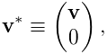 |
(2.1) |
while the representation for a point p is
 |
(2.2) |
Both classes provide a number of methods for applying rotational and affine transforms. Those used for rotations are
where R is a rotation matrix and v1 is a vector (or a point in the case of Point3d).
The methods for applying rigid or affine transforms include:
where X is a rigid or affine transform. As described above, in the case of Vector3d, these methods ignore the translational part of the transform and apply only the matrix component (R for a RigidTransform3d and A for an AffineTransform3d). In particular, that means that for a RigidTransform3d given by X and a Vector3d given by v, the method calls
produce the same result.
2.4 Spatial vectors and inertias
The velocities, forces and inertias associated with 3D coordinate frames and rigid bodies are represented using the 6 DOF spatial quantities described in Sections A.5 and A.6. These are implemented by classes in the package maspack.spatialmotion.
Spatial velocities (or twists) are implemented by Twist, which exposes its translational and angular velocity components through the publicly accessible fields v and w, while spatial forces (or wrenches) are implemented by Wrench, which exposes its translational force and moment components through the publicly accessible fields f and m.
Both Twist and Wrench contain methods for algebraic operations such as addition and scaling. They also contain transform() methods for applying rotational and rigid transforms. The rotation methods simply transform each component by the supplied rotation matrix. The rigid transform methods, on the other hand, assume that the supplied argument represents a transform between two frames fixed within a rigid body, and transform the twist or wrench accordingly, using either (A.27) or (A.29).
The spatial inertia for a rigid body is implemented by SpatialInertia, which contains a number of methods for setting its value given various mass, center of mass, and inertia values, and querying the values of its components. It also contains methods for scaling and adding, transforming between coordinate systems, inversion, and multiplying by spatial vectors.
2.5 Meshes
ArtiSynth makes extensive use of 3D meshes, which are defined in maspack.geometry. They are used for a variety of purposes, including visualization, collision detection, and computing physical properties (such as inertia or stiffness variation within a finite element model).
A mesh is essentially a collection of vertices (i.e., points) that are topologically connected in some way. All meshes extend the abstract base class MeshBase, which supports the vertex definitions, while subclasses provide the topology.
Through MeshBase, all meshes provide methods for adding and accessing vertices. Some of these include:
Vertices are implemented by Vertex3d, which defines the position of the vertex (returned by the method getPosition()), and also contains support for topological connections. In addition, each vertex maintains an index, obtainable via getIndex(), that equals the index of its location within the mesh’s vertex list. This makes it easy to set up parallel array structures for augmenting mesh vertex properties.
Mesh subclasses currently include:
- PolygonalMesh
-
Implements a 2D surface mesh containing faces implemented using half-edges.
- PolylineMesh
-
Implements a mesh consisting of connected line-segments (polylines).
- PointMesh
-
Implements a point cloud with no topological connectivity.
PolygonalMesh is used quite extensively and provides a number of methods for implementing faces, including:
The class Face implements a face as a counter-clockwise arrangement of vertices linked together by half-edges (class HalfEdge). Face also supplies a face’s (outward facing) normal via getNormal().
Some mesh uses within ArtiSynth, such as collision detection, require a triangular mesh; i.e., one where all faces have three vertices. The method isTriangular() can be used to check for this. Meshes that are not triangular can be made triangular using triangulate().
2.5.1 Mesh creation
It is possible to create a mesh by direct construction. For example, the following code fragment creates a simple closed tetrahedral surface:
However, meshes are more commonly created using either one of the factory methods supplied by MeshFactory, or by reading a definition from a file (Section 2.5.5).
Some of the more commonly used factory methods for creating polyhedral meshes include:
Each factory method creates a mesh in some standard coordinate
frame. After creation, the mesh can be transformed using the
transform(X) method, where X is either a rigid transform (
RigidTransform3d) or a more general affine
transform (AffineTransform3d).
For example, to create a rotated box centered on ![]() ,
one could do:
,
one could do:
One can also scale a mesh using scale(s), where s is a single scale factor, or scale(sx,sy,sz), where sx, sy, and sz are separate scale factors for the x, y and z axes. This provides a useful way to create an ellipsoid:
MeshFactory can also be used to create new meshes by performing boolean operations on existing ones:
2.5.2 Setting normals, colors, and textures
Meshes provide support for adding normal, color, and texture information, with the exact interpretation of these quantities depending upon the particular mesh subclass. Most commonly this information is used simply for rendering, but in some cases normal information might also be used for physical simulation.
For polygonal meshes, the normal information described here is used only for smooth shading. When flat shading is requested, normals are determined directly from the faces themselves.
Normal information can be set and queried using the following methods:
The method setNormals() takes two arguments: a set of normal vectors (nrmls), along with a set of index values (indices) that map these normals onto the vertices of each of the mesh’s geometric features. Often, there will be one unique normal per vertex, in which case nrmls will have a size equal to the number of vertices, but this is not always the case, as described below. Features for the different mesh subclasses are: faces for PolygonalMesh, polylines for PolylineMesh, and vertices for PointMesh. If indices is specified as null, then normals is assumed to have a size equal to the number of vertices, and an appropriate index set is created automatically using createVertexIndices() (described below). Otherwise, indices should have a size of equal to the number of features times the number of vertices per feature. For example, consider a PolygonalMesh consisting of two triangles formed from vertex indices (0, 1, 2) and (2, 1, 3), respectively. If normals are specified and there is one unique normal per vertex, then the normal indices are likely to be
[ 0 1 2 2 1 3 ]
As mentioned above, sometimes there may be more than one normal per vertex. This happens in cases when the same vertex uses different normals for different faces. In such situations, the size of the nrmls argument will exceed the number of vertices.
The method setNormals() makes internal copies of the specified normal and index information, and this information can be later read back using getNormals() and getNormalIndices(). The number of normals can be queried using numNormals(), and individual normals can be queried or set using getNormal(idx) and setNormal(idx,nrml). All normals and indices can be explicitly cleared using clearNormals().
Color and texture information can be set using analagous methods. For colors, we have
When specified as float[], colors are given as RGB or
RGBA values, in the range ![]() , with array lengths of 3 and 4,
respectively. The colors returned by
getColors() are always RGBA
values.
, with array lengths of 3 and 4,
respectively. The colors returned by
getColors() are always RGBA
values.
With colors, there may often be fewer colors than the number of vertices. For instance, we may have only two colors, indexed by 0 and 1, and want to use these to alternately color the mesh faces. Using the two-triangle example above, the color indices might then look like this:
[ 0 0 0 1 1 1 ]
Finally, for texture coordinates, we have
When specifying indices using setNormals, setColors, or setTextureCoords, it is common to use the same index set as that which associates vertices with features. For convenience, this index set can be created automatically using
Alternatively, we may sometimes want to create a index set that assigns the same attribute to each feature vertex. If there is one attribute per feature, the resulting index set is called a feature index set, and can be created using
If we have a mesh with three triangles and one color per triangle, the resulting feature index set would be
[ 0 0 0 1 1 1 2 2 2 ]
Note: when a mesh is modified by the addition of new features (such as faces for PolygonalMesh), all normal, color and texture information is cleared by default (with normal information being automatically recomputed on demand if automatic normal creation is enabled; see Section 2.5.3). When a mesh is modified by the removal of features, the index sets for normals, colors and textures are adjusted to account for the removal.
For colors, it is possible to request that a mesh explicitly maintain colors for either its vertices or features (Section 2.5.4). When this is done, colors will persist when vertices or features are added or removed, with default colors being automatically created as necessary.
Once normals, colors, or textures have been set, one may want to know which of these attributes are associated with the vertices of a specific feature. To know this, it is necessary to find that feature’s offset into the attribute’s index set. This offset information can be found using the array returned by
For example, the three normals associated with a triangle at index ti can be obtained using
Alternatively, one may use the convenience methods
which return the attribute values for the ![]() -th vertex of
the feature indexed by fidx.
-th vertex of
the feature indexed by fidx.
In general, the various get methods return references to internal storage information and so should not be modified. However, specific values within the lists returned by getNormals(), getColors(), or getTextureCoords() may be modified by the application. This may be necessary when attribute information changes as the simultion proceeds. Alternatively, one may use methods such as setNormal(idx,nrml) setColor(idx,color), or setTextureCoords(idx,coords).
Also, in some situations, particularly with colors and textures, it may be desirable to not have color or texture information defined for certain features. In such cases, the corresponding index information can be specified as -1, and the getNormal(), getColor() and getTexture() methods will return null for the features in question.
2.5.3 Automatic creation of normals and hard edges
For some mesh subclasses, if normals are not explicitly set, they are computed automatically whenever getNormals() or getNormalIndices() is called. Whether or not this is true for a particular mesh can be queried by the method
Setting normals explicitly, using a call to setNormals(nrmls,indices), will overwrite any existing normal information, automatically computed or otherwise. The method
will return true if normals have been explicitly set, and false if they have been automatically computed or if there is currently no normal information. To explicitly remove normals from a mesh which has automatic normal generation, one may call setNormals() with the nrmls argument set to null.
More detailed control over how normals are automatically created may be available for specific mesh subclasses. For example, PolygonalMesh allows normals to be created with multiple normals per vertex, for vertices that are associated with either open or hard edges. This ability can be controlled using the methods
Having multiple normals means that even with smooth shading, open or hard edges will still appear sharp. To make an edge hard within a PolygonalMesh, one may use the methods
which control the hardness of edges between individual vertices, specified either directly or using their indices.
2.5.4 Vertex and feature coloring
The method setColors() makes it possible to assign any desired coloring scheme to a mesh. However, it does require that the user explicity reset the color information whenever new features are added.
For convenience, an application can also request that a mesh explicitly maintain colors for either its vertices or features. These colors will then be maintained when vertices or features are added or removed, with default colors being automatically created as necessary.
Vertex-based coloring can be requested with the method
This will create a separate (default) color for each of the mesh’s vertices, and set the color indices to be equal to the vertex indices, which is equivalent to the call
where colors contains a default color for each vertex. However, once vertex coloring is enabled, the color and index sets will be updated whenever vertices or features are added or removed. Meanwhile, applications can query or set the colors for any vertex using getColor(idx), or any of the various setColor methods. Whether or not vertex coloring is enabled can be queried using
Once vertex coloring is established, the application will typically want to set the colors for all vertices, perhaps using a code fragment like this:
Similarly, feature-based coloring can be requested using the method
This will create a separate (default) color for each of the mesh’s features (faces for PolygonalMesh, polylines for PolylineMesh, etc.), and set the color indices to equal the feature index set, which is equivalent to the call
where colors contains a default color for each feature. Applications can query or set the colors for any vertex using getColor(idx), or any of the various setColor methods. Whether or not feature coloring is enabled can be queried using
2.5.5 Reading and writing mesh files
The package maspack.geometry.io supplies a number of classes for writing and reading meshes to and from files of different formats.
Some of the supported formats and their associated readers and writers include:
| Extension | Format | Reader/writer classes |
|---|---|---|
| .obj | Alias Wavefront | WavefrontReader, WavefrontWriter |
| .ply | Polygon file format | PlyReader, PlyWriter |
| .stl | STereoLithography | StlReader, StlWriter |
| .gts | GNU triangulated surface | GtsReader, GtsWriter |
| .off | Object file format | OffReader, OffWriter |
The general usage pattern for these classes is to construct the desired reader or writer with a path to the desired file, and then call readMesh() or writeMesh() as appropriate:
Both readMesh() and writeMesh() may throw I/O exceptions, which must be either caught, as in the example above, or thrown out of the calling routine.
For convenience, one can also use the classes GenericMeshReader or GenericMeshWriter, which internally create an appropriate reader or writer based on the file extension. This enables the writing of code that does not depend on the file format:
Here, fileName can refer to a mesh of any format supported by GenericMeshReader. Note that the mesh returned by readMesh() is explicitly cast to PolygonalMesh. This is because readMesh() returns the superclass MeshBase, since the default mesh created for some file formats may be different from PolygonalMesh.
2.5.6 Reading and writing normal and texture information
When writing a mesh out to a file, normal and texture information are also written if they have been explicitly set and the file format supports it. In addition, by default, automatically generated normal information will also be written if it relies on information (such as hard edges) that can’t be reconstructed from the stored file information.
Whether or not normal information will be written is returned by the method
This will always return true if any of the conditions described above have been met. So for example, if a PolygonalMesh contains hard edges, and multiple automatic normals are enabled (i.e., getMultipleAutoNormals() returns true), then getWriteNormals() will return true.
Default normal writing behavior can be overridden within the MeshWriter classes using the following methods:
where enable should be one of the following values:
- 0
-
normals will never be written;
- 1
-
normals will always be written;
- -1
-
normals will written according to the default behavior described above.
When reading a PolygonalMesh from a file, if the file contains normal information with multiple normals per vertex that suggests the existence of hard edges, then the corresponding edges are set to be hard within the mesh.
Chapter 3 Mechanical Models I
This section details how to build basic multibody-type mechanical models consisting of particles, springs, rigid bodies, joints, and other constraints.
3.1 Springs and particles
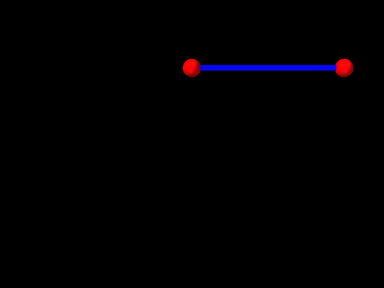
The most basic type of mechanical model consists simply of particles connected together by axial springs. Particles are implemented by the class Particle, which is a dynamic component containing a three-dimensional position state, a corresponding velocity state, and a mass. It is an instance of the more general base class Point, which is used to also implement spatial points such as markers which do not have a mass.
3.1.1 Axial springs and materials
An axial spring is a simple spring that connects two points and is
implemented by the class
AxialSpring. This is a force effector component that exerts equal and opposite forces on the
two points, along the line separating them, with a magnitude ![]() that
is a function
that
is a function ![]() of the distance
of the distance ![]() between the points,
and the distance derivative
between the points,
and the distance derivative ![]() .
.
Each axial spring is associated with an axial material,
implemented by a subclass of
AxialMaterial, that specifies
the function ![]() . The most basic type of axial material is
a LinearAxialMaterial, which
determines
. The most basic type of axial material is
a LinearAxialMaterial, which
determines ![]() according to the linear relationship
according to the linear relationship
| (3.1) |
where ![]() is the rest length and
is the rest length and ![]() and
and ![]() are the stiffness and
damping terms. Both
are the stiffness and
damping terms. Both ![]() and
and ![]() are properties of the material, while
are properties of the material, while
![]() is a property of the spring.
is a property of the spring.
Axial springs are assigned a linear axial material by default. More complex, non-linear axial materials may be defined in the package artisynth.core.materials. Setting or querying a spring’s material may be done with the methods setMaterial() and getMaterial().
3.1.2 Example: A simple particle-spring model
An complete application model that implements a simple particle-spring model is given below.
Line 1 of the source defines the package in which the model class will reside, in this case artisynth.demos.tutorial. Lines 3-8 import definitions for other classes that will be used.
The model application class is named ParticleSpring and declared to extend RootModel (line 13), and the build() method definition begins at line 15. (A no-args constructor is also needed, but because no other constructors are defined, the compiler creates one automatically.)
To begin, the build() method creates a MechModel named "mech", and then adds it to the models list of the root model using the addModel() method (lines 18-19). Next, two particles, p1 and p2, are created, with masses equal to 2 and initial positions at 0, 0, 0, and 1, 0, 0, respectively (lines 22-23). Then an axial spring is created, with end points set to p1 and p2, and assigned a linear material with a stiffness and damping of 20 and 10 (lines 24-27). Finally, after the particles and the spring are created, they are added to the particles and axialSprings lists of the MechModel using the methods addParticle() and addAxialSpring() (lines 30-32).
At this point in the code, both particles are defined to be
dynamically controlled, so that running the simulation would cause
both to fall under the MechModel’s default gravity acceleration
of ![]() . However, for this example, we want the first
particle to remain fixed in place, so we set it to be non-dynamic (line 34), meaning that the physical simulation will not
update its position in response to forces (Section
3.1.3).
. However, for this example, we want the first
particle to remain fixed in place, so we set it to be non-dynamic (line 34), meaning that the physical simulation will not
update its position in response to forces (Section
3.1.3).
The remaining calls control aspects of how the model is graphically rendered. setBounds() (line 37) increases the model’s ``bounding box'' so that by default it will occupy a larger part of the viewer frustum. The covenience method RenderProps.setSphericalPoints() is used to set points p1 and p2 to render as solid red spheres with a radius of 0.06, while RenderProps.setCylindricalLines() is used to set spring to render as a solid blue cylinder with a radius of 0.02. More details about setting render properties are given in Section 4.3.
3.1.3 Dynamic, parametric, and attached components
By default, a dynamic component is advanced through time in response to the forces applied to it. However, it is also possible to set a dynamic component’s dynamic property to false, so that it does not respond to force inputs. As shown in the example above, this can be done using the method setDynamic():
comp.setDynamic (false);
The method isDynamic() can be used to query the dynamic property.
Dynamic components can also be attached to other dynamic components (as mentioned in Section 1.2) so that their positions and velocities are controlled by the master components that they are attached to. To attach a dynamic component, one creates an AttachmentComponent specifying the attachment connection and adds it to the MechModel, as described in Section 3.5. The method isAttached() can be used to determine if a component is attached, and if it is, getAttachment() can be used to find the corresponding AttachmentComponent.
Overall, a dynamic component can be in one of three states:
- active
-
Component is dynamic and unattached. The method isActive() returns true. The component will move in response to forces.
- parametric
-
Component is not dynamic, and is unattached. The method isParametric() returns true. The component will either remain fixed, or will move around in response to external inputs specifying the component’s position and/or velocity. One way to supply such inputs is to use controllers or input probes, as described in Section 5.
- attached
-
Component is attached. The method isAttached() returns true. The component will move so as to follow the other master component(s) to which it is attached.
3.1.4 Custom axial materials
Application authors may create their own axial materials by subclassing AxialMaterial and overriding the functions
where excitation is an additional excitation signal ![]() , which
is used to implement active springs and which in particular is used to
implement axial muscles (Section 4.4), for
which
, which
is used to implement active springs and which in particular is used to
implement axial muscles (Section 4.4), for
which ![]() is usually in the range
is usually in the range ![]() .
.
The first three methods should return the values of
 |
(3.2) |
respectively, while the last method should return true if
![]() ; i.e., if it is
always equals to 0.
; i.e., if it is
always equals to 0.
3.1.5 Damping parameters
Mechanical models usually contain damping forces in addition to spring-type restorative forces. Damping generates forces that reduce dynamic component velocities, and is usually the major source of energy dissipation in the model. Damping forces can be generated by the spring components themselves, as described above.
A general damping can be set for all particles by setting the MechModel’s pointDamping property. This causes a force
| (3.3) |
to be applied to all particles, where ![]() is the value of the pointDamping and
is the value of the pointDamping and ![]() is the particle’s velocity.
is the particle’s velocity.
pointDamping can be set and queried using the MechModel methods
In general, whenever a component has a property propX, that property can be set and queried in code using methods of the form
  setPropX (T d);
  T getPropX();
where T is the type associated with the property.
pointDamping can also be set for particles individually. This property is inherited (Section 1.4.2), so that if not set explicitly, it inherits the nearest explicitly set value in an ancestor component.
3.2 Rigid bodies
Rigid bodies are implemented in ArtiSynth by the class RigidBody, which is a dynamic component containing a six-dimensional position and orientation state, a corresponding velocity state, an inertia, and an optional surface mesh.
A rigid body is associated with its own 3D spatial coordinate frame, and is a subclass of the more general Frame component. The combined position and orientation of this frame with respect to world coordinates defines the body’s pose, and the associated 6 degrees of freedom describe its ``position'' state.
3.2.1 Frame markers
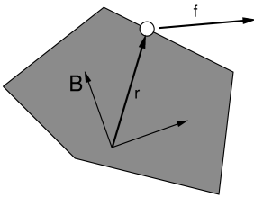
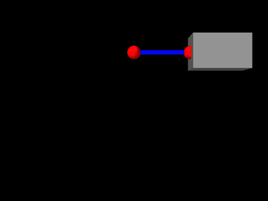
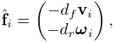
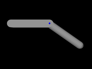
ArtiSynth makes extensive use of markers, which are (massless) points attached to dynamic components in the model. Markers are used for graphical display, implementing attachments, and transmitting forces back onto the underlying dynamic components.
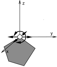
A frame marker is a marker that can be attached to a Frame, and most commonly to a RigidBody (Figure 3.2). They are frequently used to provide the anchor points for attaching springs and, more generally, applying forces to the body.
Frame markers are implemented by the class FrameMarker, which is a subclass of Point. The methods
get and set the marker’s location ![]() with respect to the frame’s
coordinate system. When a 3D force
with respect to the frame’s
coordinate system. When a 3D force ![]() is applied to the marker, it
generates a spatial force
is applied to the marker, it
generates a spatial force ![]() (Section
A.5) on the frame given by
(Section
A.5) on the frame given by
 |
(3.4) |
3.2.2 Example: A simple rigid body-spring model
A simple rigid body-spring model is defined in
artisynth.demos.tutorial.RigidBodySpring
This differs from ParticleSpring only in the build() method, which is listed below:
The differences from ParticleSpring begin
at line 9. Instead of creating a second particle, a rigid body is
created using the factory method
RigidBody.createBox(), which
takes x, y, z widths and a (uniform) density and creates a box-shaped
rigid body complete with surface mesh and appropriate mass and
inertia. As the box is initially centered at the origin, moving it
elsewhere requires setting the body’s pose, which is done using setPose(). The RigidTransform3d passed to setPose() is
created using a three-argument constructor that generates a
translation-only transform. Next, starting at line 14, a FrameMarker is created for a location ![]() relative to the
rigid body, and attached to the body using its setFrame()
method.
relative to the
rigid body, and attached to the body using its setFrame()
method.
The remainder of build() is the same as for ParticleSpring, except that the spring is attached to the frame marker instead of a second particle.
3.2.3 Creating rigid bodies
As illustrated above, rigid bodies can be created using factory methods supplied by RigidBody. Some of these include:
The bodies do not need to be named; if no name is desired, then name and can be specified as null.
In addition, there are also factory methods for creating a rigid body directly from a mesh:
These take either a polygonal mesh (Section 2.5), or a file name from which a mesh is read, and use it as the body’s surface mesh and then compute the mass and inertia properties from the specified (uniform) density.
Alternatively, one can create a rigid body directly from a constructor, and then set the mesh and inertia properties explicitly:
3.2.4 Pose and velocity
A body’s pose can be set and queried using the methods
These use a RigidTransform3d (Section
2.2) to describe the pose. Body poses are
described in world coordinates and specify the transform from body to
world coordinates. In particular, the pose for a body A specifies
the rigid transform ![]() .
.
Rigid bodies also expose the translational and rotational components of their pose via the properties position and orientation, which can be queried and set independently using the methods
The velocity of a rigid body is described using a Twist (Section 2.4), which contains both the translational and rotational velocities. The following methods set and query the spatial velocity as described with respect to world coordinates:
During simulation, unless a rigid body has been set to be parametric (Section 3.1.3), its pose and velocity are updated in response to forces, so setting the pose or velocity generally makes sense only for setting initial conditions. On the other hand, if a rigid body is parametric, then it is possible to control its pose during the simulation, but in that case it is better to set its target pose and/or target velocity, as described in Section 5.3.1.
3.2.5 Inertia and meshes
The ``mass'' of a rigid body is described by its spatial inertia (Section A.6), implemented by a SpatialInertia object, which specifies its mass, center of mass, and rotational inertia with respect to the center of mass.
Most rigid bodies are also associated with a polygonal surface mesh, which can be set and queried using the methods
The second method takes an optional fileName argument that can be set to the name of a file from which the mesh was read. Then if the model itself is saved to a file, the model file will specify the mesh using the file name instead of explicit vertex and face information, which can reduce the model file size considerably.
The inertia of a rigid body can be explicitly set using a variety of methods including
and can be queried using
In practice, it is often more convenient to simply specify a mass or a density, and then use the volume defined by the surface mesh to compute the remaining inertial values. How a rigid body’s inertia is computed is determined by its inertiaMethod property, which can be one
- Density
-
Inertia is computed from density;
- Mass
-
Inertia is computed from mass;
- Explicit
-
Inertia is set explicitly.
This property can be set and queried using
and its default value is Density. Explicitly setting the inertia using one of setInertia() methods described above will set inertiaMethod to Explicit. The method
will (re)compute the inertia using the mesh and a density value and set inertiaMethod to Density, and the method
will (re)compute the inertia using the mesh and mass value and set inertiaMethod to Mass.
Finally, the (assumed uniform) density of the body can be queried using
3.2.6 Damping parameters
As with particles, it is possible to set damping parameters for rigid bodies.
MechModel provides two properties, frameDamping and rotaryDamping, which generate a spatial force centered on each rigid body’s coordinate frame
 |
(3.5) |
where ![]() and
and ![]() are the frameDamping and rotaryDamping values, and
are the frameDamping and rotaryDamping values, and ![]() and
and ![]() are the translational
and angular velocity of the body’s coordinate frame.
The damping parameters can be set and queried using the MechModel
methods
are the translational
and angular velocity of the body’s coordinate frame.
The damping parameters can be set and queried using the MechModel
methods
For models involving rigid bodies, it is often necessary to set rotaryDamping to a non-zero value because frameDamping will provide no damping at all when a rigid body is simply rotating about its coordinate frame origin.
Frame and rotary damping can also be set for individual bodies using their own (inherited) frameDamping and rotaryDamping properties.
3.3 Joints and connectors
In a typical mechanical model, many of the rigid bodies are interconnected, either using spring-type components that exert binding forces on the bodies, or through joint-type connectors that enforce the connection using hard constraints.
3.3.1 Joints and coordinate frames
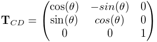
Consider two bodies A and B. The pose of body B with respect to body A
can be described by the 6 DOF rigid transform ![]() . If bodies A
and B are unconnected,
. If bodies A
and B are unconnected, ![]() may assume any possible value
and has a full six degrees of freedom. A joint between A and B
restricts the set of poses that are possible between the two bodies
and reduces the degrees of freedom available to
may assume any possible value
and has a full six degrees of freedom. A joint between A and B
restricts the set of poses that are possible between the two bodies
and reduces the degrees of freedom available to ![]() . For
simplicity, joints have their own coordinate frames for describing
their constraining actions, and then these frames are related to the
frames A and B of the associated bodies by auxiliary transformations.
. For
simplicity, joints have their own coordinate frames for describing
their constraining actions, and then these frames are related to the
frames A and B of the associated bodies by auxiliary transformations.
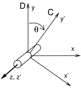
Each joint is associated with two coordinate frames C and D which move
with respect to each other as the joint moves. The allowed joint
motions therefore correspond to the allowed values of the joint transform
![]() . D is the base frame and C is the motion
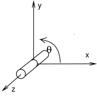
frame. For a revolute joint (Figure 3.4), C can
move with respect to D by rotating about the z axis. Other motions are
prohibited.
. D is the base frame and C is the motion
frame. For a revolute joint (Figure 3.4), C can
move with respect to D by rotating about the z axis. Other motions are
prohibited. ![]() should therefore alway have the form
should therefore alway have the form
 |
(3.6) |
where ![]() is the angle of joint rotation and is known as the joint parameter. Other joints have different parameterizations, with
the number of parameters equaling the number of degrees of freedom
available to the joint. When
is the angle of joint rotation and is known as the joint parameter. Other joints have different parameterizations, with
the number of parameters equaling the number of degrees of freedom
available to the joint. When ![]() (where
(where ![]() is the
identity transform), the parameters are all (usually) equal to zero,
and the joint is said to be in the zero state.
is the
identity transform), the parameters are all (usually) equal to zero,
and the joint is said to be in the zero state.

In practice, due to numerical errors and/or compliance in the joint,
the joint transform ![]() may
sometimes deviate from the allowed set of values dictated by the joint
type. In ArtiSynth, this is accounted for by introducing an additional
constraint frame G between D and C (Figure 3.5).
G is computed to be the nearest frame to C that lies exactly
in the joint constraint space.
may
sometimes deviate from the allowed set of values dictated by the joint
type. In ArtiSynth, this is accounted for by introducing an additional
constraint frame G between D and C (Figure 3.5).
G is computed to be the nearest frame to C that lies exactly
in the joint constraint space. ![]() is therefore a
valid transform for the joint,
is therefore a
valid transform for the joint, ![]() accommodates the error,
and the whole joint transform is given by the composition
accommodates the error,
and the whole joint transform is given by the composition
| (3.7) |
If there is no compliance or joint error, then frames G and C are the
same, ![]() , and
, and ![]() .
.
In general, each joint is attached to two rigid bodies A and B, with
frame C being fixed to body A and frame D being fixed to body B. The
restrictions of the joint transform ![]() therefore restrict the
relative poses of A and B.
therefore restrict the
relative poses of A and B.
Except in special cases, the joint coordinate frames C and D are not
coincident with the body frames A and B. Instead, they are located
relative to A and B by the transforms ![]() and
and ![]() ,
respectively (Figure 3.6).
Since
,
respectively (Figure 3.6).
Since ![]() and
and ![]() are both fixed, the pose
of B relative to A can be determined from
the joint transform
are both fixed, the pose
of B relative to A can be determined from
the joint transform ![]() :
:
| (3.8) |
(See Section A.2 for a discussion of determining transforms between related coordinate frames).
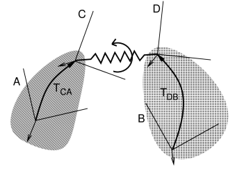
3.3.2 Creating Joints
Joint components in ArtiSynth are implemented by subclasses of BodyConnector. Some of the commonly used ones are described in Section 3.3.4.
An application creates a joint by constructing it and adding it to a MechModel. Most joints generally have a constructor of the form
which specifies the rigid bodies A and B which the joint connects,
along with the transform ![]() giving the pose of the joint base
frame D in world coordinates. Then constructor then assumes that the
joint is in the zero state, so that C and D are the same and
giving the pose of the joint base
frame D in world coordinates. Then constructor then assumes that the
joint is in the zero state, so that C and D are the same and
![]() and
and ![]() , and then computes
, and then computes
![]() and
and ![]() from
from
| (3.9) | ||||
| (3.10) |
where ![]() and
and ![]() are the poses of A and B.
The same body and transform settings can be made on an existing
joint using the method
setBodies(bodyA, bodyB, TDW).
are the poses of A and B.
The same body and transform settings can be made on an existing
joint using the method
setBodies(bodyA, bodyB, TDW).
Alternatively, if we prefer to explicitly specify ![]() or
or ![]() , then we
can determine
, then we
can determine ![]() from
from ![]() or
or ![]() using
using
| (3.11) | ||||
| (3.12) |
For example, if we know ![]() , this can be accomplished using
the following code fragment:
, this can be accomplished using
the following code fragment:
Another method,
setBodies(bodyA, TCA, bodyB, TDB), allows us to set both values of
![]() or
or ![]() explicitly. This is useful if the joint
transform
explicitly. This is useful if the joint
transform ![]() is known to be some value other than the
identity, in which case
is known to be some value other than the
identity, in which case ![]() or
or ![]() can be computed
from (3.8), where
can be computed
from (3.8), where ![]() is given by
is given by
| (3.13) |
For instance, if we know ![]() and the joint transform
and the joint transform ![]() ,
then we can compute
,
then we can compute ![]() from
from
| (3.14) |
and set up the joint as follows:
Some joint implementations provide the ability to explicitly set the
joint parameter(s) after it has been created and added to the MechModel, making it easy to ``move'' the joint to a specific
configuration. For example, RevoluteJoint provides the method
setTheta().
This causes the transform ![]() to be explicitly set to the value
implied by the joint parameters, and the pose of either body A or B is
changed to accommodate this. Whether body A or B is moved depends on
which one is the least connected to ``ground'', and other bodies that have
joint connections to the moved body are moved as well.
to be explicitly set to the value
implied by the joint parameters, and the pose of either body A or B is
changed to accommodate this. Whether body A or B is moved depends on
which one is the least connected to ``ground'', and other bodies that have
joint connections to the moved body are moved as well.
If desired, joints can be connected to only a single rigid body. In this case, the second body B is simply assumed to be ``ground'', and the coordinate frame B is instead taken to be the world coordinate frame W. The corresponding calls to the joint constructor or setBodies() take the form
or
3.3.3 Example: A simple revolute joint
A simple model showing two rigid bodies connected by a joint is defined in
artisynth.demos.tutorial.RigidBodyJoint
The build method for this model is given below:
A MechModel is created as usual at line 4. However, in this
example, we also set some parameters for it:
setGravity() is
used to set the gravity acceleration vector to ![]() instead
of the default value of
instead
of the default value of ![]() , and the frameDamping
and rotaryDamping properties (Section
3.2.6) are set to provide appropriate damping.
, and the frameDamping
and rotaryDamping properties (Section
3.2.6) are set to provide appropriate damping.
Each of the two rigid bodies are created from a mesh and a density. The meshes themselves are created using the factory methods MeshFactory.createRoundedBox() and MeshFactory.createRoundedCylinder() (lines 13 and 22), and then RigidBody.createFromMesh() is used to turn these into rigid bodies with a density of 0.2 (lines 17 and 25). The pose of the two bodies is set using RigidTransform3d objects created with x, y, z translation and axis-angle orientation values (lines 18 and 26).
The revolute joint is implemented using RevoluteJoint, which is constructed at line 32 with the joint coordinate frame D being located in world coordinates by TDW as described in Section 3.3.2.
Once the joint is created and added to the MechModel, the method
setTheta() is
used to explicitly set the joint parameter to 35 degrees. The joint
transform ![]() is then set appropriately and bodyA is moved
to accommodate this (bodyA being chosen since it is the freest
to move).
is then set appropriately and bodyA is moved
to accommodate this (bodyA being chosen since it is the freest
to move).
Finally, render properties are set starting at line 42. A revolute joint is rendered as a line segment, using the line render properties (Section 4.3), with lineStyle and lineColor set to Cylinder and BLUE, respectively, by default. The cylinder radius and length are specified by the line render property lineRadius and the revolute joint property axisLength, which are set explicitly in the code.
3.3.4 Commonly used joints
 |
 |
 |
 |
Some of the joints commonly used by ArtiSynth are shown in Figure 3.8. Each illustration shows the allowed joint motion relative to the base coordinate frame D. Clockwise from the top-left, these joints are:
- Revolute joint
-
A one DOF joint which allows rotation by an angle
 about
the z axis.
about
the z axis. - Roll-pitch joint
-
A two DOF joint, similar to the revolute joint, which allows the rotation about z to be followed by an additional rotation
 about
the (new) y axis.
about
the (new) y axis. - Spherical joint
-
A three DOF joint in which the origin remains fixed but any orientation may be assumed.
- Planar connector
-
A five DOF joint which connects a point on a single rigid body to a plane in space. The point may slide freely in the x-y plane, and the body may assume any orientation about the point.
3.4 Frame springs
Another way to connect two rigid bodies together is to use a frame spring, which is a six dimensional spring that generates restoring forces and moments between coordinate frames.
3.4.1 Frame spring coordinate frames

The basic idea of a frame spring is shown in Figure
3.9. It generates restoring forces and moments on
two frames C and D which are a function of ![]() and
and ![]() (the spatial velocity of frame D with respect to frame C).
(the spatial velocity of frame D with respect to frame C).
Decomposing forces into stiffness and damping terms, the force
![]() and moment
and moment ![]() acting on C can be expressed as
acting on C can be expressed as
| (3.15) |
where the translational and rotational forces ![]() ,
, ![]() ,
,
![]() , and
, and ![]() are general functions of
are general functions of ![]() and
and
![]() .
.
The forces acting on D are equal and opposite, so that
| (3.16) |
If frames C and D are attached to a pair of rigid bodies A and B, then
a frame spring can be used to connect them in a manner analogous to a
joint. As with joints, C and D generally do not coincide with the body
frames, and are instead offset from them by fixed transforms ![]() and
and ![]() (Figure 3.10).
(Figure 3.10).
3.4.2 Frame materials
The restoring forces (3.15) generated in a frame spring depend on the frame material associated with the spring. Frame materials are defined in the package artisynth.core.materials, and are subclassed from FrameMaterial. The most basic type of material is a LinearFrameMaterial, in which the restoring forces are determined from
where ![]() gives the small angle approximation of the
rotational components of
gives the small angle approximation of the
rotational components of ![]() with respect to the
with respect to the ![]() ,
, ![]() , and
, and
![]() axes, and
axes, and
 |
||
 |
are the stiffness and damping matrices. The diagonal values defining
each matrix are stored in the 3-dimensional vectors ![]() ,
, ![]() ,
,
![]() , and
, and ![]() which are exposed as the stiffness, rotaryStiffness, damping, and rotaryDamping properties of
the material. Each of these specifies stiffness or damping values
along or about a particular axis. Specifying different values for
different axes will result in anisotropic behavior.
which are exposed as the stiffness, rotaryStiffness, damping, and rotaryDamping properties of
the material. Each of these specifies stiffness or damping values
along or about a particular axis. Specifying different values for
different axes will result in anisotropic behavior.
Other frame materials offering nonlinear behaviour may be defined in artisynth.core.materials.
3.4.3 Creating frame springs
Frame springs are implemented by the class
FrameSpring. Creating a frame
spring generally involves instantiating this class, and then setting
the material, the bodies A and B, and the transforms ![]() and
and
![]() .
.
A typical construction sequence might look like this:
The material is set using
setMaterial().
The example above uses a LinearFrameMaterial, created with a
constructor that sets ![]() ,
, ![]() ,
, ![]() , and
, and ![]() to uniform
isotropic values specified by kt, kr, dt, and dr.
to uniform
isotropic values specified by kt, kr, dt, and dr.
The bodies and transforms can be set in the same manner as for joints
(Section 3.3.2), with the
methods
setFrames(bodyA,bodyB,TDW)
and
setFrames(bodyA,TCA,bodyB,TDB)
assuming the role of the setBodies() methods used for joints.
The former takes D specified in world coordinates and computes
![]() and
and ![]() assuming that there is no initial spring
displacement (i.e., that
assuming that there is no initial spring
displacement (i.e., that ![]() ), while the latter allows
), while the latter allows
![]() and
and ![]() to be specified explicitly with
to be specified explicitly with ![]() assuming whatever value is implied.
assuming whatever value is implied.
Frame springs and joints are often placed together, using the same
transforms ![]() and
and ![]() , with the spring providing
restoring forces to help keep the joint within prescribed bounds.
, with the spring providing
restoring forces to help keep the joint within prescribed bounds.
As with joints, a frame spring can be connected to only a single body, by specifying frameB as null. Frame B is then taken to be the world coordinate frame W.
3.4.4 Example: Two bodies connected by a frame spring
A simple model showing two simplified lumbar vertebrae, modeled as rigid bodies and connected by a frame spring, is defined in
artisynth.demos.tutorial.LumbarFrameSpring
The definition for the entire model class is shown here:
For convenience, the code to create and add each vertebrae is wrapped into the method addBone() defined at lines 27-32. This method takes two arguments: the MechModel to which the bone should be added, and the name of the bone. Surface meshes for the bones are located in .obj files located in the directory ../mech/geometry relative to the source directory for the model itself. ArtisynthPath.getSrcRelativePath() is used to find a proper path to this directory given the model class type (LumbarFrameSpring.class), and this is stored in the static string geometryDir. Within addBone(), the directory path and the bone name are used to create a path to the bone mesh itself, which is in turn used to create a PolygonalMesh (line 28). The mesh is then used in conjunction with a density to create a rigid body which is added to the MechModel (lines 29-30) and returned.
The build() method begins by creating and adding a MechModel, specifying a low value for gravity, and setting the rigid
body damping properties frameDamping and rotaryDamping (lines 37-41). (The damping parameters are needed
here because the frame spring itself is created with no damping.)
Rigid bodies representing the vertebrae lumbar1 and lumbar2 are then created by calling addBone() (lines 44-45),
lumbar1 is translated by setting the origin of its pose to
![]() , and lumbar2 is set to be fixed by making
it non-dynamic (line 47).
, and lumbar2 is set to be fixed by making
it non-dynamic (line 47).
At this point in the construction, if the model were to be loaded, it would appear as in Figure 3.12. To change the viewpoint to that seen in Figure 3.11, we rotate the entire model about the x axis (line 50). This is done using transformGeometry(X), which transforms the geometry of an entire model using a rigid or affine transform. This method is described in more detail in Section 4.7.
The frame spring is created and added at lines 54-59, using the methods described in Section 3.4.3, with frame D set to the (initial) pose of lumbar1.
Render properties are set starting at line 62. By default, a frame spring renders as a pair of red, green, blue coordinate axes showing frames C and D, along with a line connecting them. The line width and the color of the connecting line are controlled by the line render properties lineWidth and lineColor, while the length of the coordinate axes is controlled by the special frame spring property axisLength.
To run this example in ArtiSynth, select All demos > tutorial > LumbarFrameSpring from the Models menu. The model should load and initially appear as in Figure 3.11. Running the model (Section 1.5.3) will cause lumbar1 to fall slightly under gravity until the frame spring arrests the motion. To get a sense of the spring’s behavior, one can interactively apply forces to lumbar1 using the pull manipulator (see the section ``Pull Manipulator'' in the ArtiSynth User Interface Guide).
3.5 Attachments
ArtiSynth provides the ability to rigidly attach dynamic components to other dynamic components, allowing different parts of a model to be connected together. Attachments are made by adding to a MechModel special attachment components that manage the attachment physics as described briefly in Section 1.2.
3.5.1 Point attachments
Point attachments allow particles and other point-based components to be attached to other, more complex components, such as frames, rigid bodies, or finite element models (Section 6.4). Point attachments are implemented by creating attachment components that are instances of PointAttachment. Modeling applications do not generally handle the attachment components directly, but instead create them implicitly using the following MechModel method:
This attaches a point p1 to any component which implements the interface PointAttachable, indicating that it is capable creating an attachment to a point. Components that implement PointAttachable currently include rigid bodies, particles, and finite element models. The attachment is created based on the the current position of the point and component in question. For attaching a point to a rigid body, another method may be used:
This attaches p1 to body at the point loc specified in body coordinates. Finite element attachments are discussed in Section 6.4.
3.5.2 Example: model with particle attachments
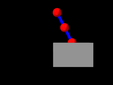
A model illustrating particle-particle and particle-rigid body attachments is defined in
artisynth.demos.tutorial.ParticleAttachment
and most of the code is shown here:
The code is very similar to ParticleSpring and RigidBodySpring described in Sections 3.1.2 and 3.2.2, except that two convenience methods, addParticle() and addSpring(), are defined at lines 1-15 to create particles and spring and add them to a MechModel. These are used in the build() method to create four particles and two springs (lines 24-29), along with a rigid body box (lines 31-34). As with the other examples, particle p1 is set to be non-dynamic (line 36) in order to fix it in place and provide a ground.
The attachments are added at lines 39-40, with p2 attached to
p3 and p4 connected to the box at the location ![]() in box coordinates.
in box coordinates.
Finally, render properties are set starting at line 43. In this example, point and line render properties are set for the entire MechModel instead of individual components. Since render properties are inherited, this will implicitly set the specified render properties in all sub-components for which these properties are not explicitly set (either locally or in an intermediate ancestor).
3.5.3 Frame attachments
Frame attachments allow rigid bodies and other frame-based components to be attached to other components, including frames, rigid bodies, or finite element models (Section 6.6). Frame attachments are implemented by creating attachment components that are instances of FrameAttachment.
As with point attachments, modeling applications do not generally handle frame attachment components directly, but instead create and add them implicitly using the following MechModel methods:
These attach frame to any component which implements the interface FrameAttachable, indicating that it is capable of creating an attachment to a frame. Components that implement FrameAttachable currently include frames, rigid bodies, and finite element models. For the first method, the attachment is created based on the the current position of the frame and component in question. For the second method, the attachment is created so that the initial pose of the frame (in world coordinates) is described by TFW.
Once a frame is attached, it will be in the attached state, as described in Section 3.1.3. Frame attachments can be removed by calling
While it is possible to create composite rigid bodies using FrameAttachments, this is much less computationally efficient (and less accurate) than creating a single rigid body through mesh merging or similar techniques.
3.5.4 Example: model with frame attachments
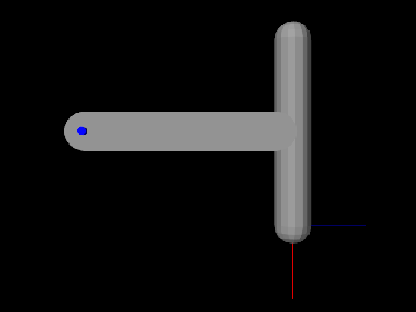
A model illustrating rigidBody-rigidBody and frame-rigidBody attachments is defined in
artisynth.demos.tutorial.FrameBodyAttachment
Most of the code is identical to that for RigidBodyJoint as described in Section 3.3.3, except that the joint is further to the left and connects bodyB to ground, rather than to bodyA, and the initial pose of bodyA is changed so that it is aligned vertically. bodyA is then connected to bodyB, and an auxiliary frame is created and attached to bodyA, using code at the end of the build() method as shown here:
To run this example in ArtiSynth, select All demos > tutorial > FrameBodyAttachment from the Models menu. The model should load and initially appear as in Figure 3.13. The frame attached to bodyA is visible in the lower right corner. Running the model (Section 1.5.3) will cause both bodies to fall and swing about the joint under gravity.
Chapter 4 Mechanical Models II
This section provides additional material on building basic multibody-type mechanical models.
4.1 Simulation control properties
Both RootModel and MechModel contain properties that control the simulation behavior. One of the most important of these is maxStepSize. By default, simulation proceeds using the maxStepSize value defined for the root model. A MechModel (or any other type of Model) contained in the root model’s models list may also request a smaller step size by specifying a smaller value for its own maxStepSize property. For all models, the maxStepSize may be set and queried using
Another important simulation property is integrator in MechModel, which determines the type of integrator used for the physics simulation. The value type of this property is the enumerated type MechSystemSolver.Integrator, for which the following values are currently defined:
- ForwardEuler
-
First order forward Euler integrator. Unstable for stiff systems.
- SymplecticEuler
-
First order symplectic Euler integrator, more energy conserving that forward Euler. Unstable for stiff systems.
- RungeKutta4
-
Fourth order Runge-Kutta integrator, quite accurate but also unstable for stiff systems.
- ConstrainedBackwardEuler
-
First order backward order integrator. Generally stable for stiff systems.
- Trapezoidal
-
Second order trapezoidal integrator. Generally stable for stiff systems, but slightly less so than ConstrainedBackwardEuler.
The term ``Unstable for stiff systems'' means that the integrator is likely to go unstable in the presence of ``stiff'' systems, which typically include systems containing finite element models, unless the simulation step size is set to an extremely small value. The default value for integrator is ConstrainedBackwardEuler.
Stiff systems tend to arise in models containing interconnected deformable elements, for which the step size should not exceed the propagation time across the smallest element, an effect known as the Courant-Friedrichs-Lewy (CFL) condition. Larger stiffness and damping values decrease the propagation time and hence the allowable step size.
Another MechModel simulation property is stabilization, which controls the stabilization method used to correct drift from position constraints and correct interpenetrations due to collisions. The value type of this property value is the enumerated type MechSystemSolver.PosStabilization, which presently has two values:
- GlobalMass
-
Uses only a diagonal mass matrix for the MLCP that is solved to determine the position corrections. This is the default method.
- GlobalStiffness
-
Uses a stiffness-corrected mass matrix for the MLCP that is solved to determine the position corrections. Slower than GlobalMass, but more likely to produce stable results, particularly for problems involving FEM collisions.
4.2 Units
ArtiSynth is primarily ``unitless'', in the sense that it does not
define default units for the fundamental physical quantities of time,
length, and mass. Although time is
generally understood to be in seconds, and often declared as such in
method arguments and return values, there is no hard requirement that
it be interpreted as seconds. There are no assumptions at all
regarding length and mass. Some components may have default parameter
values that reflect a particular choice of units, such as MechModel’s default gravity value of ![]() , which is
associated with the MKS system, but these values can always be
overridden by the application.
, which is
associated with the MKS system, but these values can always be
overridden by the application.
Nevertheless, it is important, and up to the application developer to
ensure, that units be consistent. For example, if one decides to
switch length units from meters to centimeters (a common choice),
then all units involving length will have to be scaled appropriately.
For example, density, whose fundamental units are ![]() , where
, where ![]() is mass and
is mass and
![]() is distance, needs to be scaled by
is distance, needs to be scaled by ![]() , or
, or ![]() , when
converting from meters to centimeters.
, when
converting from meters to centimeters.
Table 4.1 lists a number of common physical quantities used in ArtiSynth, along with their associated fundamental units.
| unit | fundamental units | |
|---|---|---|
| time | ||
| distance | ||
| mass | ||
| velocity | ||
| acceleration | ||
| force | ||
| work/energy | ||
| torque | same as energy (somewhat counter intuitive) | |
| angular velocity | ||
| angular acceleration | ||
| rotational inertia | ||
| pressure | ||
| Young’s modulus | ||
| Poisson’s ratio | 1 | no units; it is a ratio |
| density | ||
| linear stiffness | ||
| linear damping | ||
| rotary stiffness | same as torque | |
| rotary damping | ||
| mass damping | used in FemModel | |
| stiffness damping | used in FemModel |
4.2.1 Scaling units
For convenience, many ArtiSynth components, including MechModel, implement the interface ScalableUnits, which provides the following methods for scaling mass and distance units:
A call to one of these methods should cause all physical quantities within the component (and its descendants) to be scaled as required by the fundamental unit relationships as shown in Table 4.1.
Converting a MechModel from meters to centimeters can therefore be easily done by calling
As an example, adding the following code to the end of the build() method in RigidBodySpring (Section 3.2.2)
will scale the distance units by 100 and print the values of various quantities before and after scaling. The resulting output is:
It is important not to confuse scaling units with scaling the actual geometry or mass. Scaling units should change all physical quantities so that the simulated behavior of the model remains unchanged. If the distance-scaled version of RigidBodySpring shown above is run, it should behave exactly the same as the non-scaled version.
4.3 Render properties
All ArtiSynth components that are renderable maintain a property renderProps, which stores a RenderProps object that contains a number of subproperties used to control an object’s rendered appearance.
In code, the renderProps property for an object can be set or queried using the methods
Render properties can also be set in the GUI by selecting one or more components and the choosing Set render props ... in the right-click context menu. More details on setting render properties through the GUI can be found in the section ``Render properties'' in the ArtiSynth User Interface Guide.
For many components, the default value of renderProps is null; i.e., no RenderProps object is assigned by default and render properties are instead inherited from ancestor components further up the hierarchy. The reason for this is because RenderProps objects are fairly large (many kilobytes), and so assigning a unique one to every component could consume too much memory. Even when a RenderProps object is assigned, most of its properties are inherited by default, and so only those properties which are explicitly set will differ from those specified in ancestor components.
4.3.1 Render property taxonomy
In general, the properties in RenderProps are used to control the color, size, and style of the three primary rendering primitives: faces, lines, and points. Table 4.2 contains a complete list. Values for the shading, faceStyle, lineStyle and pointStyle properties are defined using the following enumerated types: Renderer.Shading, Renderer.FaceStyle, Renderer.PointStyle, and Renderer.LineStyle. Colors are specified using java.awt.Color.
| property | purpose | usual default value |
| visible | whether or not the component is visible | true |
| alpha | transparency for diffuse colors (range 0 to 1) | 1 (opaque) |
| shading | shading style: (FLAT, SMOOTH, METAL, NONE) | FLAT |
| shininess | shininess parameter (range 0 to 128) | 32 |
| specular | specular color components | null |
| faceStyle | which polygonal faces are drawn (FRONT, BACK, FRONT_AND_BACK, NONE) | FRONT |
| faceColor | diffuse color for drawing faces | GRAY |
| backColor | diffuse color used for the backs of faces. If null, faceColor is used. | null |
| drawEdges | hint that polygon edges should be drawn explicitly | false |
| colorMap | color mapping properties (see Section 4.3.3) | null |
| normalMap | normal mapping properties (see Section 4.3.3) | null |
| bumpMap | bump mapping properties (see Section 4.3.3) | null |
| edgeColor | diffuse color for edges | null |
| edgeWidth | edge width in pixels | 1 |
| lineStyle: | how lines are drawn (CYLINDER, LINE, or SPINDLE) | LINE |
| lineColor | diffuse color for lines | GRAY |
| lineWidth | width in pixels when LINE style is selected | 1 |
| lineRadius | radius when CYLINDER or SPINDLE style is selected | 1 |
| pointStyle | how points are drawn (SPHERE or POINT) | POINT |
| pointColor | diffuse color for points | GRAY |
| pointSize | point size in pixels when POINT style is selected | 1 |
| pointRadius | sphere radius when SPHERE style is selected | 1 |
To increase and improve their visibility, both the line and point primitives are associated with styles (CYLINDER, SPINDLE, and SPHERE) that allow them to be rendered using 3D surface geometry.
Exactly how a component interprets its render properties is up to the component (and more specifically, up to the rendering method for that component). Not all render properties are relevant to all components, particularly if the rendering does not use all of the rendering primitives. For example, Particle components use only the point primitives and AxialSpring components use only the line primitives. For this reason, some components use subclasses of RenderProps, such as PointRenderProps and LineRenderProps, that expose only a subset of the available render properties. All renderable components provide the method createRenderProps() that will create and return a RenderProps object suitable for that component.
4.3.2 Setting render properties
When setting render properties, it is important to note that the value returned by getRenderProps() should be treated as read-only and should not be used to set property values. For example, applications should not do the following:
This can cause problems for two reasons. First, getRenderProps() will return null if the object does not currently have a RenderProps object. Second, because RenderProps objects are large, ArtiSynth may try to share them between components, and so by setting them for one component, the application my inadvertently set them for other components as well.
Instead, RenderProps provides a static method for each property that can be used to set that property’s value for a specific component. For example, the correct way to set pointColor is
One can also set render properties by calling setRenderProps() with a predefined RenderProps object as an argument. This is useful for setting a large number of properties at once:
For setting each of the color properties within RenderProps, one can use either Color objects or float[] arrays of length 3 giving the RGB values. Specifically, there are methods of the form
as well as the static methods
where XXX corresponds to Point, Line, Face, Edge, and Back. For Edge and Back, both color and rgb can be given as null to clear the indicated color. For the specular color, the associated methods are
Note that even though components may use a subclass of RenderProps internally, one can always use the base RenderProps class to set values; properties which are not relevant to the component will simply be ignored.
Finally, as mentioned above, render properties are inherited. Values set high in the component hierarchy will be inherited by descendant components, unless those descendants (or intermediate components) explicitly set overriding values. For example, a MechModel maintains its own RenderProps (and which is never null). Setting its pointColor property to RED will cause all point-related components within that MechModel to be rendered as red except for components that set their pointColor to a different property.
There are typically three levels in a MechModel component hierarchy at which render properties can be set:
-
•
The MechModel itself;
-
•
Lists containing components;
-
•
Individual components.
For example, consider the following code:
Setting the MechModel render property pointColor to BLUE will cause all point-related items to be rendered blue by default. Setting the pointColor render property for the particle list (returned by mech.particles()) will override this and cause all particles in the list to be rendered green by default. Lastly, setting pointColor for p3 will cause it to be rendered as red.
4.3.3 Texture mapping
Render properties can also be set to apply texture mapping to objects containing polygonal meshes in which texture coordinates have been set. Supported is provided for color, normal and bump mapping, although normal and bump mapping are only available under the OpenGL 3 version of the ArtiSynth renderer.
Texture mapping is controlled through the colorMap, normalMap, and bumpMap properties of RenderProps. These are composite properties with a default value of null, but applications can set them to instances of ColorMapProps, NormalMapProps, and BumpMapProps, respectively, to provide the source images and parameters for the associated mapping. The two most important properties exported by all of these MapProps objects are:
- enabled
-
A boolean indicating whether or not the mapping is enabled.
- fileName
-
A string giving the file name of the supporting source image.
NormalMapProps and BumpMapProps also export scaling,
which scales the x-y components of the normal map or the depth of the
bump map. Other exported properties control mixing with underlying
colors, and how texture coordinates are both filtered and managed when
they fall outside the canonical range ![]() . Full details on
texture mapping and its support by the ArtiSynth renderer are given in
the ``Rendering'' section of the Maspack
Reference Manual.
. Full details on
texture mapping and its support by the ArtiSynth renderer are given in
the ``Rendering'' section of the Maspack
Reference Manual.
To set up a texture map, one creates an instance of the appropriate MapProps object and uses this to set either the colorMap, normalMap, or bumpMap property of RenderProps. For a specific renderable, the map properties can be set using the static methods
When initializing the PropMaps object, it is often sufficient to just set enabled to true and fileName to the full path name of the source image. Normal and bump maps also often require adjustment of their scaling properties. The following static methods are available for setting the enabled and fileName subproperties within a renderable:
Normal and bump mapping only work under the OpenGL 3 version of the ArtiSynth viewer, and also do not work if the shading property of RenderProps is set to NONE or FLAT.
Texture mapping properties can be set within ancestor nodes of the component hierarchy, to allow file names and other parameters to be propagated throughout the hierarchy. However, when this is done, it is still necessary to ensure that the corresponding mapping properties for the relevant descendants are non-null. That’s because mapping properties themselves are not inherited; only their subproperties are. If a mapping property for any given object is null, the associated mapping will be disabled. A non-null mapping property for an object will be created automatically by calling one of the setXXXEnabled() methods listed above. So when setting up ancestor-controlled mapping, one may use a construction like this:
      RenderProps.setColorMap (ancestor, tprops);
      RenderProps.setColorMapEnabled (descendant0, true);
      RenderProps.setColorMapEnabled (descendant1, true);
Then colorMap sub-properties set within ancestor will be inherited by descendant0 and descendant1.
As indicated above, texture mapping will only be applied to components containing rendered polygonal meshes for which appropriate texture coordinates have been set. Determining such texture coordinates that produce appropriate results for a given source image is often non-trivial; this so-called ``u-v mapping problem'' is difficult in general and is highly dependent on the mesh geometry. ArtiSynth users can handle the problem of assigning texture coordinates in several ways:
-
•
Use meshes which already have appropriate texture coordinates defined for a given source image. This generally means that mesh is specified by a file that contains the required texture coordinates. The mesh should then be read from this file (Section 2.5.5) and then used in the construction of the relevant components. For example, the application can read in a mesh containing texture coordinates and then use it to create a RigidBody via the method RigidBody.createFromMesh().
-
•
Use a simple mesh object with predefined texture coordinates. The class MeshFactory provides the methods
PolygonalMesh createRectangle (width, height, xdivs, ydivs, addTextureCoords);PolygonalMesh createSphere (radius, nslices, nlevels, addTextureCoords)which create rectangular and spherical meshes, along with canonical canonical texture coordinates if addTextureCoords is true. Coordinates generated by createSphere() are defined so that
 and
and  map to the spherical coordinates
  (at
the south pole) and
(at
the south pole) and  (at the north pole). Source images can
be relatively easy to find for objects with canonical coordinates.
(at the north pole). Source images can
be relatively easy to find for objects with canonical coordinates. -
•
Compute custom texture coordinates and set them within the mesh using setTextureCoords().
An example where texture mapping is applied to spherical meshes to make them appear like tennis balls is defined in
artisynth.demos.tutorial.SphericalTextureMapping
and listing for this is given below:
The build() method uses the internal method createBall() to generate three rigid bodies, each defined using a spherical mesh that has been created with MeshFactory.createSphere() with addTextureCoords set to true. The remainder of the build() method sets up the render properties and the texture mappings. Two texture mappings are defined: a color mapping and bump mapping, based on the images TennisBallColorMap.jpg and TennisBallBumpMap.jpg (Figure 4.2), both located in the subdirectory data relative to the demo source file. PathFinder.expand() is used to determine the full data folder name relative to the source directory. For the bump map, it is important to set the scaling property to adjust the depth amplitude to relative to the sphere radius.
 |
 |
Color mapping is applied to balls 0 and 2, and bump mapping to balls 1 and 2. To illustrate setting mapping properties in an ancestor component, the color mapping is arranged by setting the colorMap render property of the MechModel, and then, as described above, enabling color mapping within the individual balls.
To run this example in ArtiSynth, select All demos > tutorial > SphericalTextureMapping from the Models menu. The model should load and initially appear as in Figure 4.1. Note that if ArtiSynth is run with the legacy OpenGL 2 viewer (command line option -GLVersion 2), bump mapping will not be supported and will not appear.
4.4 Point-to-point muscles
Point-to-point muscles are a simple type of component in biomechanical models that provide muscle-activated forces acting along a line between two points. ArtiSynth provides this through Muscle, which is a subclass of AxialSpring that generates an active muscle force in response to its excitation property. The excitation property can be set and queried using the methods
4.4.1 Muscle materials
As with AxialSprings, Muscle components use an
AxialMaterial to compute the
applied force ![]() in response to the muscle’s length
in response to the muscle’s length
![]() , length velocity
, length velocity ![]() , and excitation signal
, and excitation signal ![]() . Usually the
force is the sum of a passive component plus an active
component that arises in response to the excitation signal.
. Usually the
force is the sum of a passive component plus an active
component that arises in response to the excitation signal.
The default AxialMaterial for a Muscle is SimpleAxialMuscle, which is essentially an activated version of LinearAxialMaterial and which computes a simple force according to
| (4.1) |
where ![]() and
and ![]() are stiffness and damping terms,
are stiffness and damping terms, ![]() is the
excitation value, and
is the
excitation value, and ![]() is the maximum excitation force.
is the maximum excitation force.
![]() ,
, ![]() and
and ![]() are exposed through the properties stiffness, damping, and maxForce.
are exposed through the properties stiffness, damping, and maxForce.
More complex muscle materials are typically used for biomechanical
modeling applications, generally with non-linear passive terms and
active terms that depend on the muscle length ![]() . Some of those
available in ArtiSynth include
ConstantAxialMuscle,
BlemkerAxialMuscle,
PaiAxialMuscle, and
PeckAxialMuscle.
. Some of those
available in ArtiSynth include
ConstantAxialMuscle,
BlemkerAxialMuscle,
PaiAxialMuscle, and
PeckAxialMuscle.
4.4.2 Example: Muscle attached to a rigid body
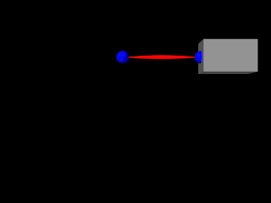
A simple model showing a single muscle connected to a rigid body is defined in
artisynth.demos.tutorial.SimpleMuscle
This model is identical to RigidBodySpring described in Section 3.2.2, except that the code to create the spring is replaced with code to create a muscle with a SimpleAxialMuscle material:
Also, so that the muscle renders differently, the rendering style for lines is set to SPINDLE using the convenience method
To run this example in ArtiSynth, select All demos > tutorial > SimpleMuscle from the Models menu. The model should load and initially appear as in Figure 4.3. Running the model (Section 1.5.3) will cause the box to fall and sway under gravity. To see the effect of the excitation property, select the muscle in the viewer and then choose Edit properties ... from the right-click context menu. This will open an editing panel that allows the muscle’s properties to be adjusted interactively. Adjusting the excitation property using the adjacent slider will cause the muscle force to vary.
4.5 Collision Handling
Collision handling in ArtiSynth is implemented by a collision handling mechanism build into MechModel. Collisions are disabled by default, but can be enabled between rigid and deformable bodies (finite element models in particular), and more generally between any body that implements the interface Collidable.
It is important to understand that collision handling is both computationally expensive and, due to it’s discontinuous nature, less accurate than other aspects of the simulation. ArtiSynth therefore provides a number of ways to selectively control collision handling between different pairs of bodies.
Collision handling is also challenging because if collisions are
enabled among ![]() objects, then one needs to be able to easily specify
the characteristics of up to
objects, then one needs to be able to easily specify
the characteristics of up to ![]() collision interactions, while
also managing the fact that these interactioons are highly transient.
In ArtiSynth, collision handling is done by a
CollisionManager that is a
sub-component of each
MechModel. The collision
manager maintains default collision behaviors among certain groups of
collidable objects, while also allowing the user to override the
default behaviors by setting override behaviors for specific component
pairings.
collision interactions, while
also managing the fact that these interactioons are highly transient.
In ArtiSynth, collision handling is done by a
CollisionManager that is a
sub-component of each
MechModel. The collision
manager maintains default collision behaviors among certain groups of
collidable objects, while also allowing the user to override the
default behaviors by setting override behaviors for specific component
pairings.
4.5.1 Enabling collisions in code
Collisions can be enabled as either a default behavior between all bodies, a default behavior between certain groups of bodies, or a specific override behavior between individual pairs of bodies.
This section describes how to enable collisions in code. However, it is also possible to set some aspects of collision behavior interactively within the ArtiSynth GUI. See the section ``Collision handling'' in the ArtiSynth User Interface Guide.
The default collision behavior between all collidables can be controlled using two methods:
In the first method, enabled is true or false depending on whether collisions are enabled, and mu is the coefficient of Coulomb (or dry) friction. The mu value is ignored if enabled is false. In the second method, behavior is a CollisionBehavior object that specifies both enabled and mu, along with other, more detailed collision properties (see Section 4.5.3). In addition, a default collision behavior can be set for generic groups of collidables using
where group0 and group1 are static instances of the special Collidable subclass Collidable.Group that represents the groups described in Table 4.3. The groups Collidable.Rigid and Collidable.Deformable denote collidables that are rigid (such as RigidBody) or deformable (such as FEM models like FemModel3d). (If a collidable is deformable, then its isDeformable() method returns true.) The group Collidable.AllBodies denotes both rigid and deformable bodies, and Collidable.Self is used to enabled self-collision. which is described in greater detail in Section 4.5.4.
| Collidable group | description |
|---|---|
| Collidable.Rigid | rigid collidables (e.g., rigid bodies) |
| Collidable.Deformable | deformable collidables (e.g, FEM models) |
| Collidable.AllBodies | rigid and deformable collidables |
| Collidable.Self | enables self-intersection for composite deformable collidables |
| Collidable.All | rigid and deformable collidables and self-intersection |
A call to one of the setDefaultCollisionBehavior() methods will override the effects of previous calls. So for instance, the code sequence
will initially enable collisions between all bodies with a friction coefficient of 0, then disable collisions between deformable and rigid bodies, and finally re-enable collisions between all bodies with a friction coefficient of 0.2.
The default collision behavior between any pair of collidable groups can be queried using
For this call, group0 and group1 are restricted to the primary groups Collidable.Rigid, Collidable.Deformable, and Collidabe.Self, since individual behaviors are not maintained for the composite groups Collidable.AllBodies and Collidable.All.
In addition to default behaviors, overriding behaviors for individual collidables or pairs of collidables can be controlled using
where collidable0 is an individual collidable component (such as a rigid body or FEM model), and collidable1 is either another individual component, or one of the groups of Table 4.3. For example, the calls
will enable collisions between bodA and all deformable collidables (with friction 0.1), as well as femB and all deformable and rigid collidables (with friction 0.0), while specifically disabling collisions between bodA and femB.
The setCollisionBehavior() methods work by adding a CollisionBehavior object to the collision manager as a sub-component. With setCollisionBehavior(collidable0,collidable1,behavior), the behavior object is created and supplied by the application. With setCollisionBehavior(enable,mu), the behavior object is created automatically and returned by the method. Once an override behavior has been specified, then it can be queried using
This method will return null if no override behavior for the pair in questions has been previously set using one of the setCollisionBehavior() methods.
Because behaviors are proper components, it is not permissible to add them to the collision manager twice. Specifically, the following will produce an error:
   CollisionBehavior behav = new CollisionBehavior();
   behav.setDrawIntersectionContours (true);
   mesh.setCollisionBehavior (col0, col1, behav);
   mesh.setCollisionBehavior (col2, col3, behav); // ERROR
However, if desired, a new behavior can be created from an existing one:
   CollisionBehavior behav = new CollisionBehavior();
   behav.setDrawIntersectionContours (true);
   mesh.setCollisionBehavior (col0, col1, behav);
   behav = new CollisionBehavior(behav);
   mesh.setCollisionBehavior (col2, col3, behav); // OK
To determine the collision behavior (default or override) that actually controls a specific pair of collidables, one may use the method
where collidable0 and collidable1 must both be specific collidable components and cannot be a group (such as Collidable.Rigid or Collidable.All). If one of the collidables is a compound collidable (Section 4.5.4), or has a collidability setting (Section 4.5.5) that prevents collisions, there may be no consistent acting behavior, in which case the method returns null.
Collision behaviors take priority over each other in the following order:
-
1.
behaviors specified using setCollisionBehavior() involving two specific collidables.
-
2.
behaviors specified using setCollisionBehavior() involving one specific collidable and a group of collidables (indicated by a Collidable.Group), with later specifications taking priority over earlier ones.
-
3.
default behaviors specified using setDefaultCollisionBehavior().
An override behavior specified with setCollisionBehavior() can later be removed using
and all override behaviors in a MechModel can be removed with
Note that this latter call does not remove default behaviors specified with setDefaultCollisionBehavior().
Note: It is usually necessary to ensure that collisions are disabled between adjacent bodies connected by joints, since otherwise these would be forced into a state of permanent collision.
4.5.2 Example: Collision with a plane
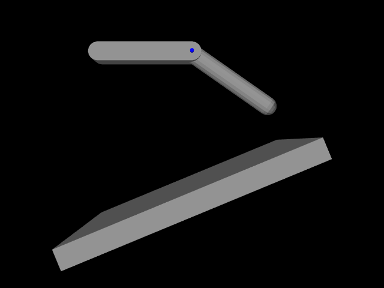
A simple model illustrating collision between two jointed rigid bodies and a plane is defined in
artisynth.demos.tutorial.JointedCollide
This model is simply a subclass of RigidBodyJoint that overrides the build() method to add an inclined plane and enable collisions between it and the two connected bodies:
The superclass build() method called at line 3 creates everything contained in RigidBodyJoint. The remaining code then alters that model: bodyB is set to be dynamic (line 5) so that it will fall freely, and an inclined plane is created from a thin box that is translated and rotated and then set to be be non-dynamic (lines 8-11). Finally, collisions are enabled by setting the default collision behavior (line 14), and then specifically disabling collisions between bodyA and bodyB (line 15). As indicated above, the latter step is necessary because the joint would otherwise keep the two bodies in a permanent state of collision.
4.5.3 Collision behaviors
As mentioned above, the CollisionBehavior objects described above can be used to control other aspects of the contact and collision beyond friction and enabling. In particular, a CollisionBehavior exports the following properties:
- enabled
-
A boolean that determines if collisions are enabled.
- friction
-
A double giving the coefficient of Coulomb friction, typically in the range
![[0,0.5]](mi/mi154.png) . The default value is 0. Setting friction to a
non-zero value increases the simulation time, since extra constraints
must be added to the system to accommodate the friction.
. The default value is 0. Setting friction to a
non-zero value increases the simulation time, since extra constraints
must be added to the system to accommodate the friction. - penetrationTol
-
A double controlling the amount of interpenetration that is permitted in order to ensure contact stability (see Section 4.6.3). If not specified, the system will inherit this property from the MechModel, which computes a default penetration tolerance based on the overall size of the model.
- compliance
-
A double which adds a compliance (inverse stiffness) to the collision behavior, so that the contact has a ``springiness''. The default value for this is 0 (no compliance).
- damping
-
A double which, if compliance is non-zero, specifies a damping to accompany the compliant behavior. The default value is 0. When compliance is specified, it is usually necessary to set the damping to a non-zero value to prevent bouncing.
- collisionPointTol
-
A double which, for contacts between rigid bodies, specifies a minimum distance between contact points that is used to reduce the number of contacts. If not explicitly specified, the system computes a default value for this based on the overall size of the model.
- reduceConstraints
-
A boolean which, if true, indicates that the system should try to reduce the number of contacts between deformable bodies with limited degrees of freedom, so that the resulting contact problem is not ill-conditioned. The default value is false.
- method
-
An instance of CollisionBehavior.Method that controls how the contact constraints for the collision response are generated. There are several methods available, and some are experimental. The more standard methods are:
Method Constraint generation VERTEX_PENETRATION constraints generated from interpenetrating vertices CONTOUR_REGION constraints generated from planes fit to each mesh contact region INACTIVE no constraints generated These are described in more detail in Section 4.6.1.
- colliderType
-
An instance of CollisionManager.ColliderType that specifies the underlying mechanism used to determine the collision information between two meshes. The choice of collider may restrict which collision methods (described above) are allowed. Collider types available at present include:
Type Description AJL_CONTOUR uses mesh intersection contour to find penetrating regions and vertices TRI_INTERSECTION uses triangle intersections to find penetrating regions and vertices SIGNED_DISTANCE uses a signed distance field to find penetrating vertices These are described in more detail in Section 4.6.1.
In addition to the above, CollisionBehavior exports other properties that control the rendering of collisions (Section 4.6.4).
It should be noted that most collision behavior properties are also properties of the MechModel’s collision manager, which can be accessed in code using getCollisionManager() (or graphically via the navigation panel). Since collision behaviors are sub-components of the collision manager, properties set in the collision manager will be inherited by any behaviors for which they have not been explicitly set. This is the easiest way to specify behavior properties generally, as for example:
Some other properties, like penetrationTol, are properties not of the collision manager, but of the MechModel, and so can be set globally there.
To set collision properties in a more fine-grained manner, one can either call setDefaultCollisionBehavior() or setCollisionBehavior() with an appropriately set CollisionBehavior object:
For behaviors that are already set, one may use getDefaultCollisionBehavior() or getCollisionBehavior() to obtain the behavior and then set the desired properties directly:
Note however that getDefaultCollisionBehavior() only works for Collidable.Rigid, Collidable.Deformable, and Collidable.Self, and that getCollisionBehavior() only works for a collidable pair that has been previously specified with setCollisionBehavior(). One may also use getActingCollisionBehavior() (described above) to obtain the behavior (default or otherwise) responsible for a specific pair of collidables, although in some instances no such single behavior exists and the method will then return null.
4.5.4 Self-collision and collidable hierarchies
At present, ArtiSynth does not support the detection or handling of self-collision within single meshes. However, self-collision can still be effected by allowing a collidable to have multiple sub-collidables and then enabling collisions between some or all of these.
Any descendant component of a Collidable A which is itself Collidable is considered to be a sub-collidable of A. Certain types of components maintain sub-collidables by default. For example, some components (such as finite element models; Section 6) maintain a list of meshes in a child component list named meshes; these can be used to implement self-collision as described below. A collidable that contains sub-collidables is known as a compound collidable, and its isCompound() method will return true. Likewise, if a component is a sub-collidable, then its getCollidableAncestor()) method will return its nearest collidable ancestor.
A collidable does not need to be an immediate child component of a collidable A in order to be a sub-collidable of A; it need only be a descendant of A.
At present, collidable hierarchies are assumed to have a depth no greater than one (i.e., no sub-collidable is itself a compound collidable), and also sub-collidables are assumed to have the same type (rigid or deformable) as the ancestor.
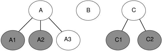
In general, an ArtiSynth model will contain a collection of collidables, some of which are compound and others which are solitary (Figure 4.5). Within a collection of collidables:
-
•
Actual collisions happen only between leaf collidables; compound collidables are used only for grouping purposes.
-
•
Leaf collidables are also instances of the sub-interface CollidableBody, which provides the additional information needed to actually determine collisions and compute the response (Section 4.6).
-
•
By default, the sub-collidables of a compound component A will only collide among themselves if self-collision is specified for A (via either a default or override collision behavior). If self-collision is specified for A, then collisions may occur only among those sub-collidables for which internal collisions are enabled. Internal collisions are enabled for a collidable if its collidable property (Section 4.5.5) is set to either ALL or INTERNAL.
-
•
Self-collision is also only possible among the sub-collidables of A if A is itself deformable; i.e., its isDeformable() method returns true.
-
•
Sub-collidables may collide with collidables outside their hierarchy if their collidable property is set to either ALL or EXTERNAL.
-
•
Collision among specific pairs of sub-collidables may also be explicitly enabled or disabled with an override behavior set using one of the setCollisionBehavior() methods.
-
•
Specifying a collision behavior among two compound collidables A and B which are not within the same hierarchy will cause that behavior to be specified among all sub-collidables of A and B whose collidable property enables the collision.
Subject to the above conditions, self-collisions can be enabled among the sub-collidables of all deformable collidables by calling
or, for a specific collidable C, by calling either
For a more complete example, refer to Figure 4.5, assume that components A, B and C are deformable, and that self-collision is allowed among those sub-collidables which are shaded gray (A1 and A2 for A, B1 and B2 for B). Then:
4.5.5 Collidability
Each collidable component maintains a collidable property (which can be queried using getCollidable()) which specifically enables or disables the ability of that collidable to collide with other collidables.
The collidable property value is of the enumerated type Collidable.Collidability, which has four possible settings:
- OFF
-
All collisions disabled: the collidable will not collide with anything.
- INTERNAL
-
Internal (self) collisions enabled: the collidable may only collide with other Collidables with which it shares a common ancestor.
- EXTERNAL
-
External collisions enabled: the collidable may only collide with other Collidables with which it does not share a common ancestor.
- ALL
-
All collisions (both self and external) enabled: the collidable may collide with any other Collidable.
Note that collidability only enables collisions. In order for collisions to actually occur between two collidables, a default or override collision behavior must also be specified for them in the MechModel.
4.5.6 Collision response
Sometimes, an application may wish to know details about the collision interactions between a specific collidable and one or more other collidables. These details may include items such as contact forces or the penetration regions between the opposing meshes. Applications can track this information by creating CollisionResponse components for the collidables in question and adding them to the MechModel using setCollisionResponse():
An alternate version of setCollisionResponse() creates the response component internally and returns it:
During every simulation step, the MechModel will update its response components to reflect the current collision conditions between the associated collidables.
The first collidable specified for a collision response must be a specific collidable component, while the second may be either another collidable or a group of collidables represented by a Collidable.Group:
When a compound collidable is specified, the response component will collect collision information for all its sub-collidables.
If desired, applications can also instantiate responses themselves and add them to the collision manager:
However, as with behaviors, the same response cannot be added to an application twice:
The complete set of methods for managing collision responses are similar to those for behaviors,
where getCollisionResponse() and clearCollisionResponse() respectively return and clear response components that have been previously set using one of the setCollisionResponse() methods.
Information that can be queried by a CollisionResponse component includes whether or not the collidable is in collision, contact impulses acting on the vertices of the colliding meshes, the penetration regions of each mesh associated with the collision, and the underlying CollisionHandler objects that maintain the contact constraints between each colliding mesh. This information may be queried with the following methods:
A typical usage scenario for collision responses is to create them before the simulation is run, possibly in the root model build() method, and then query them when the simulation is running, such from the apply() method of a Monitor ( Section 5.3). For example, in the root model build() method, the response coule be created with the call
and then used in some runtime code as follows:
If for some reason it is difficult to store a reference to the response between its construction and its use, then getCollisionResponse() can be used to retrieve it:
4.5.7 Nested MechModels
It is possible in ArtiSynth for one MechModel to contain other nested MechModels within its component hierarchy. This raises the question of how collisions within the nested models are controlled. The general rule for this is the following:
The collision behavior for two collidables colA and colB is determined by whatever behavior (either default or override) is specified by the lowest MechModel in the component hierarchy that contains both colA and colB.
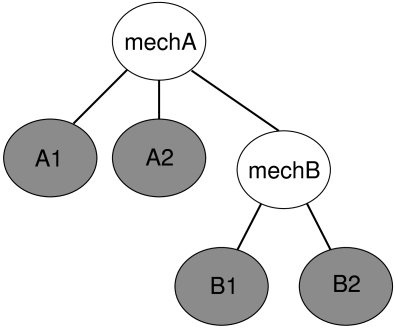
For example, consider Figure 4.6 where we have a MechModel (mechB) containing collidables B1 and B2, nested within another MechModel (mechA) containing collidables A1 and A2. Then consider the following code fragment:
The first line enables default collisions within mechB (with
![]() ), controlling the interaction between B1 and B2.
However, collisions are still disabled within mechA, meaning
A1 and A2 will not collide either with each other or with
B1 or B2. The second line enables collisions between B1 and any other body within mechA (i.e., A1 and
A2), while the third line disables collisions between B1
and A1. Finally, the fourth line results in an error, since
B1 and B2 are both contained within mechB and so
their collision behavior cannot be controlled from mechA.
), controlling the interaction between B1 and B2.
However, collisions are still disabled within mechA, meaning
A1 and A2 will not collide either with each other or with
B1 or B2. The second line enables collisions between B1 and any other body within mechA (i.e., A1 and
A2), while the third line disables collisions between B1
and A1. Finally, the fourth line results in an error, since
B1 and B2 are both contained within mechB and so
their collision behavior cannot be controlled from mechA.
While it is not legal to specify a specific behavior for collidables contained a MechModel from a higher level MechModel, it is legal to create collision response components for the same pair within both models. So the following code fragment would be allowed and would create response components in both mechA and mechB:
4.6 Collision Implementation and Rendering
As mentioned in Section 4.5.4, the leaf collidables which actually provide collision interaction are also instances of CollidableBody, which provides methods returning the information needed to compute collisions and their response. Some of these methods include:
getCollisionMesh() returns the surface mesh which is used as the basis for collision. If hasDistanceGrid() returns true, then the body also maintains a signed distance grid for the mesh, which can be obtained using getDistanceGrid() and is used by the collider type SIGNED_DISTANCE (Section 4.6.1).
4.6.1 Collision methods and collider types
The ArtiSynth collision mechanism works by using a collider (described further below) to find the intersections between the surface meshes of each collidable object. Information provided by the collider is then used to generate contact constraints, according to a collision method, that prevent further collision and resolve any existing interpenetration.
Collision methods are specified by collision behavior’s method property, which is an instance of CollisionBehavior.Method, as mentioned in Section 4.5.3. Some of the standard methods are:
- VERTEX_PENETRATION
-
A contact constraint is generated for each mesh vertex that interpenetrates the other mesh, with the normal direction determined by finding the nearest point on the opposing mesh. This method is the default for collisions involving deformable bodies which have enough degrees of freedom (DOF) that the resulting number of contacts does not overconstrain the system. Using this method for collisions between rigid bodies, or low DOF deformable bodies, will generally result in an overconstrained system unless the constraints are either regularized using compliance or constraint reduction is enabled.
- CONTOUR_REGION
-
Contact constraints are generated by fitting a plane to each mesh contact region and then projecting the region onto that plane. Constraints are then created from points on the perimeter of this projection, with the normal direction being given by the plane normal. This is the default method for collision between rigid bodies or low DOF deformable bodies. Trying to use this method for FEM-based deformable bodies will result in an error.
- DEFAULT
-
Selects the method most appropriate depending on the DOFs of the colliding bodies and whether they are rigid or deformable . This is the default setting.
- INACTIVE
-
No constraints are generated. This will result in no collision response.
The contact information used by the collision method is generated by a collider. Colliders are described by instances of CollisionManager.ColliderType and can be specified by the colliderType property in either the collision manager (as the default), or in the collision behavior for a specific pair of collidables. Since different colliders may provide different collision information, some colliders may restrict the type of collision method that may be used.
Three collider types are presently supprted:
- AJL_CONTOUR
-
A bounding-box hierachy is used to locate all triangle intersections between the two surface meshes, and the intersection points are then connected to find the (piecewise linear) intersection contours. The surface meshes must (at present) be triangular, closed, and manifold. The contours are then used to identity the contact regions on each surface mesh, which can be used to determine interpenetrating vertices and contact area. Intersection contours and the contact constraints generated from them are shown in Figure 4.7.
- TRI_INTERSECTION
-
A legacy method which also uses a bounding-box hierachy to locate all triangle intersections between the two surface meshes. However, contours are not generated. Instead, contact regions are estimated by grouping the intersection points together, and penetrating vertices are computed separately using point-mesh distance queries based on the bounding-box hierachy. This latter step requires interating over all mesh vertices, which may be slow for large meshes.
- SIGNED_DISTANCE
-
Uses a grid-based signed distance field on one mesh to quickly determine the penetrating vertices of the opposite mesh, along with the penetration distance and normals. This is only available for collidable pairs where at least one of the bodies maintains a signed distance grid which can be obtained using getDistanceGrid(). Advantages include speed (often an order of magnitude faster that the colliders based on triangle intersection) and the fact that the opposite mesh does not have to be triangular, closed, or manifold. However, signed distance fields can (at present) only be computed for fixed meshes, and so at least one colliding body must be rigid. The signed distance field also does not yield contact region information, and so the collision method is restricted to VERTEX_PENETRATION. Contacts generated from a signed distance field are illustrated in Figure Figure 4.8.
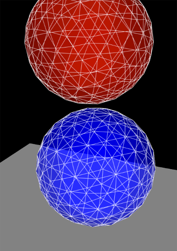 |
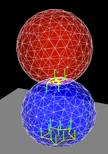 |
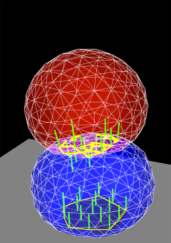 |
|
|
|
|
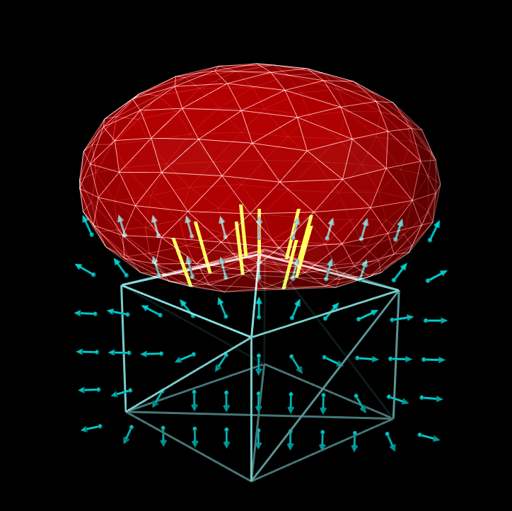
4.6.2 Configuring and rendering signed distance grids
As mentioned above, bodies which maintain signed distance grids expose these using the hasDistanceGrid() and getDistanceGrid() methods. By default, these grids are created automatically on-demand within an axis-aligned bounding volume for the mesh. The cell resolution (number of cells along the x, y, z directions) is also choosen automatically. However, in some cases it may be necessary to control the cell resolution more precisely. If the body supports the interface HasDistanceGrid, this provides a set of methods for controlling the cell resolution:
setDistanceGridRes() explicity sets the grid resolution, which is the number of grid cells along the x, y, z axes. If any of these values are specified as 0, then all values are set to zero and the resolution is determined instead by the maximum cell resolution returned by getDistanceGridMaxRes(), which specifies the number of cells along the maximum x, y, z direction, with the cell counts along the other directions adjusted to maintain a uniform cell size.
HasDistanceGrid also provides methods to support the rendering of the signed distance grid:
setRenderDistanceGrid() enables or disables grid rendering. By default, grids are rendered by drawing each cell vertex along with the associated normal (which is the numeric derivative of the distance field), using the point and line render properties for the component. In some cases, it may be desirable to restrict which vertices are drawn. This can be done using setDistanceGridRenderRanges(), which takes a string argument containing vertex render ranges for the x, y, and z axes. A vertex render range may be either * (all vertices), n:m (vertices in the index range n to m, inclusive), or n (vertices only at index n). For example:
4.6.3 Penetration tolerance and limitations
ArtiSynth’s attempt to separate colliding bodies at the end of each time step may cause a jittering behavior around the colliding area, as the surface collides, separates, and re-collides. This can usually be stabilized by maintaining a certain interpenetration distance during contact. This distance is controlled by the MechModel property penetrationTol. ArtiSynth attempts to compute a suitable default value for this property, but for some applications it may be necessary to control the value explicitly using the MechModel methods
Another issue is that because ArtiSynth currently uses static collision detection, it is possible for objects that are fast enough or thin enough to completely pass through each other in one simulation step. This means that for thin objects, it is important to keep the step size small enough to prevent such undetected interpenetration.
4.6.4 Contact rendering
As mentioned above, CollisionBehavior also contains properties that can enable and control the rendering of artifacts associated with the contact. These include intersection contours and contact points and normals, as described below. Colors, line widths, and other graphical details are controlled by the generic render properties (Section 4.3) of the collision manager, or by render properties which can be set individually within the behavior components.
By default, contact rendering is disabled. To enable it, one must set the collision manager to be visible, which can be done using a code fragment like the following:
RenderProps.setVisible (mechModel.getCollisionManager(), true);
Specific properties of CollisionBehavior that control contract rendering include:
- drawIntersectionContours
-
Boolean value requesting drawing of the intersection contours between meshes, using the edgeWidth and edgeColor render properties.
- drawIntersectionPoints
-
Boolean value requesting drawing of the interpenetrating vertices on each mesh, using the pointStyle, pointSize, pointRadius, and pointColor render properties.
- drawContactNormals
-
Boolean value requesting drawing of the normals associated with each contact constraint, using the lineStyle, lineWidth, lineRadius, and lineColor render properties. The length of the normals is controlled by the contactNormalLen property of the collision manager, which will be set to an appropriate default value if not set explicitly.
- drawPenetrationDepth
-
Integer value requesting drawing of the interpenetration depth of one mesh with respect to the other. The integer value should be either -1, 0 or 1, where -1 disables this feature and 0 or 1 select depth drawing for either the first or second mesh associated with the collision behavior.
Penetration depth is drawn using a ``heat map'' type of rendering, where the depth value range is controlled using the penetrationDepthRange property (see next item) and depth values are mapped onto colors using the colorMap property of the collision manager. The depth map itself is drawn as a patch formed from the mesh’s penetrating faces, using vertex coloring where the color at each vertex is determined by the penetration depth. An example is given in Section 4.6.6.
- penetrationDepthRange
-
Composite property of the type ScalarRange that controls the range used for depth rendering. Sub properties include interval, which gives the depth range to be used for the depth map, and updating, which specifies how this range should be updated: FIXED (no updating), AUTO_EXPAND (range is expanded as depth increases), and AUTO_FIT (range is reset every step).
Most of the above properties are also present in the CollisionManager, from which they are inherited by all behaviors that do not set them explicitly.
Generic render properties within the collision manager can be set in the same way as the visibility, using the RenderProps methods presented in Section 4.3.2:
As mentioned above, generic render properties can also be set individually for specific behaviors. This can be done using code fragments like this:
To access these properties on a read-only basis, one can do
4.6.5 Example: Rendering normals and contours
A simple model showing contact rendering is defined in
artisynth.demos.tutorial.BallPlateCollide
This shows a rigid sphere colliding with a plane, while rendering the resulting contact normals in red and the intersection contours in blue.
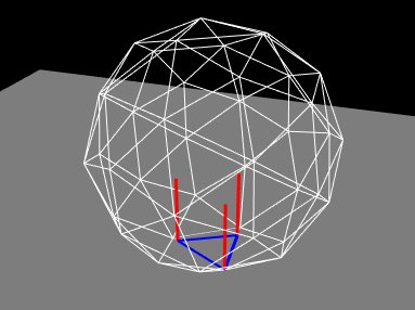
The complete source code is shown below:
To run this example in ArtiSynth, select All demos > tutorial > BallPlateCollide from the Models menu. When run, the ball will collide with the plate and the contact normals and collision contours will be drawn as shown in Figure 4.9.
4.6.6 Example: Rendering penetration depth
As described above, it is possible to use the drawPenetrationDepth property to render the extent to which one mesh interpenetrates another. A simple example of this is defined in
artisynth.demos.tutorial.PenetrationRender
which displays the penetration depth of one hemispherical mesh with respect to another.
The complete source code is shown below:
To improve visibility, the example uses two rigid bodies, each created from an open hemispherical mesh using the method createHemiBody() (lines 31-46). Because this example is strictly graphical, the bodies are set to be non-dynamic so that they can be moved around using the viewer’s graphical dragger fixtures (see the section ``Geometric Manipulation'' in the ArtiSynth User Interface Guide). Rendering properties for each body are set at lines 66-67 and 72-75, with the top body being rendered as a wireframe to improve visibility.
Lines 79-84 create and set a collision behavior between the two bodies with penetration depth rendering enabled. Because for this example we want to show only the penetration and don’t want a collision response, we set the collision method to be Method.INACTIVE. The updating of the penetration range is also set to AUTO_FIT so that it will be recomputed at every time step. At line 82, the collider type used by the collision manager is set to ColliderType.AJL_CONTOUR, since this is needed for depth rendering. Other rendering properties are set for the collision manager at lines 90-105, including a custom color map that varies between CREAM (the color of the mesh) for no penetration and dark red for maximum penetration.
At line 109, a color bar is created and added to the scene, using the method createColorBar() (lines 49-58), to explicitly show the depth that corresponds to the different colors. The color bar is given the same color map that is used to render the depth. Since the depth range is updated every time step, it is also necessary to update the corresponding labels in the color bar. This is done by overriding the root model’s prerender() method (lines 113-130), where we obtain the collision behavior between the two bodies, and use its depth range to update the color bar labels. References to the color bar, MechModel, and bodies are obtained using the CompositeComponent methods get() and findComponent(). This is more robust that storing these references in member variables, since the latter would be lost if the model is saved to and reloaded from a file.
To run this example in ArtiSynth, select All demos > tutorial > PenetrationRender from the Models menu. When run, the meshes will collide and render the penetration depth of the bottom mesh, as shown in Figure 4.10.
4.7 Transforming geometry
Certain ArtiSynth components, including MechModel, implement the interface TransformableGeometry, which allows the geometric transformation of the component’s attributes (such as meshes, points, frame locations, etc.), along with its descendant components. The interface provides the method
where X is an AffineTransform3dBase that may be either a RigidTransform3d or a more general AffineTransform3d (Section 2.2).
transformGeometry(X) can be used to translate, rotate, shear or scale components. It can be applied to an entire model or individual components. Unlike scaleDistance(), it actually changes the physical geometry and so may change the simulation behavior. For example, applying transformGeometry() to a RigidBody will cause the shape of its mesh to change, which will change its mass if its inertiaDensity property is set to Density. Figure 4.11 shows a simplified illustration of both rigid and affine transformations being applied to a model.
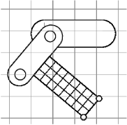 |
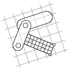 |
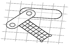 |
The example below shows how to apply a transformation to a model in code. In it, a MechModel is first scaled by the factors 1.5, 2, and 3 along the x, y, and z axes, and then flipped upside down using a RigidTransform3d that rotates it by 180 degrees about the x axis:
4.7.1 Nonlinear transformations
The TransformableGeometry interface also supports general, non-linear geometric transforms. This can be done using a GeometryTransformer, which is an abstract class for performing general transformations. To apply such a transformation to a component, one can create and initialize an appropriate subclass of GeometryTransformer to perform the desired transformation, and then apply it using the static transform method of the utility class TransformGeometryContext:
At present, the following subclasses of GeometryTransformer are available:
- RigidTransformer
-
Implements rigid 3D transformations.
- AffineTransformer
-
Implements affine 3D transformations.
- FemGeometryTransformer
-
Implements a general transformation, using the deformation field induced by a finite element model.
TransformGeometryContext also supplies the following convenience methods to apply transformations to components or collections of components:
The last three of these methods create an instance of either RigidTransformer or AffineTransformer for the supplied AffineTransform3dBase. In fact, most TransformableGeometry components implement their transformGeometry(X) method as follows:
The FemGeometryTransformer class is derived from the class DeformationTransformer, which uses the single method getDeformation() to obtain deformation field information at a specified reference position:
If the deformation field is described by ![]() , then
for a given reference position
, then
for a given reference position ![]() (in undeformed coordinates),
this method should return the deformed position
(in undeformed coordinates),
this method should return the deformed position ![]() and the deformation gradient
and the deformation gradient
 |
(4.2) |
evaluated at ![]() .
.
FemGeometryTransformer obtains
![]() and
and ![]() from a
FemModel3d (see Section
6) whose elemental rest positions enclose the
components to be transformed, using the fact that a finite element
model creates an implied piecewise-smooth deformation field as it
deviates from its rest position. For each reference point
from a
FemModel3d (see Section
6) whose elemental rest positions enclose the
components to be transformed, using the fact that a finite element
model creates an implied piecewise-smooth deformation field as it
deviates from its rest position. For each reference point ![]() needed
by the transformation process, FemGeometryTransformer finds the
FEM element whose rest volume encloses
needed
by the transformation process, FemGeometryTransformer finds the
FEM element whose rest volume encloses ![]() , and then uses the
corresponding shape function coordinates to compute
, and then uses the
corresponding shape function coordinates to compute ![]() and
and ![]() from the element’s deformation. If the FEM model does not
enclose
from the element’s deformation. If the FEM model does not
enclose ![]() , the nearest element is used to determine the shape
function coordinates (however, this calculation becomes less accurate and
meaningful the farther
, the nearest element is used to determine the shape
function coordinates (however, this calculation becomes less accurate and
meaningful the farther ![]() is from the FEM model). Transformations based
on FEM models are further illustrated in Section
4.7.2, and by Figure
4.13. Full details on ArtiSynth finite
element models are given in Section 6.
is from the FEM model). Transformations based
on FEM models are further illustrated in Section
4.7.2, and by Figure
4.13. Full details on ArtiSynth finite
element models are given in Section 6.
Besides FEM models, there are numerous other ways to create deformation fields, such as radial basis functions, thin plate splines, etc. Some of these may be more appropriate for a particular application and can provide deformations that are globally smooth (as opposed to piecewise smooth). It should be relatively easy for an application to create its own subclass of DeformationTransformer to implement the deformation of choice by overriding the single getDeformation() method.
4.7.2 Example: the FemModelDeformer class
An FEM-based geometric transformation of a MechModel is facilitated by the class FemModelDeformer, which one can add to an existing RootModel to transform the geometry of a MechModel already located within that RootModel. FemModelDeformer subclasses FemModel3d to include a FemGeometryTransformer, and provides some utility methods to support the transformation process.
A FemModelDeformer can be added to a RootModel by adding the following code fragment to the end of the build() method:
When the deformer is created, its constructor searches the specified RootModel to locate the first top-level MechModel. It then creates a hexahedral FEM grid around this model, with maxn specifying the number of cells along the maximum dimension. Material and mass properties of the model are computed automatically from the underlying MechModel dimensions (but can be altered if necessary after construction). When added to the RootModel, the deformer becomes another top-level model that can be deformed independently of the MechModel to create the required deformation field, as described below. It also supplies application-defined menu items that appear under the Application menu in the ArtiSynth menu bar (see Section 5.5). The deformer’s createControlPanel() can also be used to create a ControlPanel (Section 5.1) that controls the visibility of the FEM model and the dynamic behavior of both it and the MechModel.
An example is defined in
artisynth.demos.tutorial.DeformedJointedCollide
where the JointedCollide example of Section 4.5.2 is extended to include a FemModelDeformer using the code described above.
To load this example in ArtiSynth, select All demos > tutorial > DeformedJointedCollide from the Models menu. The model should load and initially appear as in Figure 4.12, where the control panel appears on the right.
The underlying MechModel (or "model") can now be transformed by first deforming the FEM model (or "grid") and then using the resulting deformation field to effect the transformation:
-
1.
Make the model non-dynamic and the grid dynamic by unchecking model dynamic and checking grid dynamic in the control panel. This means that when simulation is run, the model will be inert while the grid will respond physically.
-
2.
Deform the grid using simulation. One easy way to do this is to fix certain nodes, generally on or near the grid boundary, and then move some of these using the translation or transrotator tool while simulation is running. To fix a set of nodes, select them in the viewer, choose Edit properties ... from the right-click context menu, and then uncheck their dynamic property. To easily select a large number of nodes without also selecting model components or grid elements, one can specify FemNode in the selection filter widget. (See the sections ``Manipulation Tools'' and ``Selection filtering'' in the ArtiSynth User Interface Guide.)
-
3.
After the grid has been deformed, choose deform from the Application menu in the ArtiSynth toolbar to transform the model. Afterwards, the transformation can be undone by choosing undo, and the grid can be reset by choosing reset grid.
-
4.
To run the deformed model after the transformation, it should again be made dynamic by checking model dynamic in the control panel. The itself grid can be made non-dynamic, and it and/or its nodes can be made invisible by unchecking grid visible and/or grid nodes visible in the control panel.
The result of a possible deformation is shown in Figure 4.13.
 |
 |
Note: FemModelDeformer is not intended to provide a general purpose solution to non-linear geometric transformations. Rather, it is mainly intended to illustrate the capabilities of GeometryTransformer and the TransformableGeometry interface.
4.7.3 Implementation and behavior
As indicated above, the management of transforming the geometry for one or more components is handled by the TransformGeometryContext class. The transform operations themselves are carried out by this class’s apply() method, which (a) assembles all the components that need to be transformed, (b) performs the actual transform operations, (c) invokes any required updating actions on other components, and finally (d) notifies parent components of the change using a GeometryChangeEvent.
To support this, ArtiSynth components which implement TransformableGeometry must also supply the methods
The first method, addTransformableDependencies(context,flags), is called in step (a) to add to the context any additional components which should be transformed along with this component. This includes any descendants which should be transformed, since the transformation of these should not generally be done within transformGeometry(gtr,context,flags).
The second method, transformGeometry(gtr,context,flags), is called in step (b) to perform the actual transformation on this component. It should use the supplied geometry transformer gtr to transform its attributes, as well as context to query what other components are also being transformed and to request any needed updating actions to be called in step (c). The flags argument specifies conditions associated with the transformation, which at the moment may currently include:
- TG_SIMULATING
-
The system is currently simulating, and therefore it may not be desirable to transform all attributes;
- TG_ARTICULATED
-
Rigid body articulation constraints should be enforced as the transform proceeds.
Full details for all this are given in the documentation for TransformGeometryContext.
The transforming behavior of a component is up to its implementing method, but the following rules are generally observed:
-
1.
Transformable descendants are also transformed, by using addTransformableDependencies() to add them to the context as described above;
-
2.
When the nodes of an FEM model (Section 6) are transformed, the rest positions are also transformed if the system is not simulating (i.e., if the TG_SIMULATING flag is not set). This also causes the mass of the adjacent nodes to be recomputed from the densities of the adjacent elements;
-
3.
When dynamic components are transformed, any attachments and constraints associated with them are updated appropriately, but only if the system is not simulating. Non-transforming dynamic components that are attached to transforming components as slaves are generally updated so as to follow the transforming components to which they are attached.
4.7.4 Use in model registration
Transforming model geometry can obviously be used as part of the process of creating subject-specific biomechanical and anatomical models. However, registration will generally require more that geometric transformation, since other properties, such as material stiffnesses, densities, and maximum forces will generally need to be adjusted as well. As a specific example, when applying a geometric transform to a model containing AxialSprings, the restLength properties of the springs will be unchanged, whereas the initial lengths may be, resulting in a different applied forces and physical behavior.
4.8 General component arrangements
As discussed in Section 1.1.5 and elsewhere, a MechModel provides a number of predefined child components for storing particles, rigid bodies, springs, constraints, and other components. However, applications are not required to store their components in these containers, and may instead create any sort of component arrangement desired.
For example, suppose that one wishes to create a biomechanical model of both the right and left human arms, consisting of bones, point-to-point muscles, and joints. The standard containers supplied by MechModel would require that all the components be placed within the following containers:
Instead of this, one may wish to set up a more appropriate component hierarchy, such as
To do this, the application build() method can create the necessary hierarchy and then populate it with whatever components are desired. Before simulation begins (or whenever the model structure is changed), the MechModel will recursively traverse the component hierarchy and update whatever internal structures are needed to run the simulation.
4.8.1 Container components
The generic class ComponentList can be used as a container for model components of a specific type. It can be created using a declaration of the form
where Type is the class type of the components and name is the name for the container. Once the container is created, it should be added to the MechModel (or another internal container) and populated with child components of the specified type. For example,
creates two containers named "parts" and "frames" for storing components of type Particle and Frame, respectively, and adds them to a MechModel referenced by mech.
In addition to ComponentList, applications may use several "specialty" container types which are subclasses of ComponentList:
- RenderableComponentList
-
A subclass of ComponentList, that has its own set of render properties which can be inherited by its children. This can be useful for compartmentalizing render behavior. Note that it is not necessary to store renderable components in a RenderableComponentList; components stored in a ComponentList will be rendered too.
- PointList
-
A RenderableComponentList that is optimized for rendering points, and also contains its own pointDamping property that can be inherited by its children.
- PointSpringList
-
A RenderableComponentList designed for storing point-based springs. It contains a material property that specifies a default axial material that can be used by its children.
- AxialSpringList
-
A PointSpringList that is optimized for rendering two-point axial springs.
If necessary, it is relatively easy to define one’s own customized list by subclassing one of the other list types. One of the main reasons for doing so, as suggested above, is to supply default properties to be inherited by the list’s descendants.
A component list which declares ModelComponent as its type can
be used to store any type of component, including other
component lists. This allows the creation of arbitrary component
hierarchies. Generally either
ComponentList<ModelComponent> or
RenderableComponentList<ModelComponent> are
best suited to implement hierarchical groupings.
4.8.2 Example: a net formed from balls and springs
A simple example showing an arrangement of balls and springs formed into a net is defined in
artisynth.demos.tutorial.NetDemo
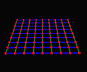
The build() method and some of the supporting definitions for this example are shown below.
The build() method begins by creating a MechModel in the usual way (lines 29-30). It then creates a net composed of a set of balls arranged as a uniform grid in the x-y plane, connected by a set of green colored springs running parallel to the y axis and a set of blue colored springs running parallel to the x axis. These are arranged into a component hierarchy of the form
using containers created at lines 37-42. The balls are then created and added to balls (lines 45-56), the springs are created and added to greenSprings and blueSprings (lines 59-71), and the containers are added to the MechModel at lines 74-77. The balls along the edges parallel to the y axis are fixed. Render properties are set at lines 80-83, with the colors for greenSprings and blueSprings being explicitly set to dark green and blue.
MechModel, along with other classes derived from ModelBase, enforces reference containment. That means that all components referenced by components within a MechModel must themselves be contained within the MechModel. This condition is checked whenever a component is added directly to a MechModel or one of its ancestors. This means that the components must be added to the MechModel in an order that ensures any referenced components are already present. For example, in the NetDemo example above, adding the particle list after the spring list would generate an error.
To run this example in ArtiSynth, select All demos > tutorial > NetDemo from the Models menu. The model should load and initially appear as in Figure 4.14. Running the model will cause the net to fall and sway under gravity. When the ArtiSynth navigation panel is opened and expanded, the component hierarchy will appear as in Figure 4.15. While the standard MechModel containers are still present, they are not displayed by default because they are empty.
4.8.3 Adding containers to other models
In addition to MechModel, application-defined containers can be added to any model that inherits from ModelBase. This includes RootModel and FemModel. However, at the present time, components added to such containers won’t do anything, other than be rendered in the viewer if they are Renderable.
Chapter 5 Simulation Control
This section describes different devices which an application may use to control the simulation. These include control panels to allow for the interactive adjustment of properties, as well as agents which are applied every time step. Agents include controllers and input probes to supply and modify input parameters at the beginning of each time step, and monitors and output probes to observe and record simulation results at the end of each time step.
5.1 Control Panels
A control panel is an editing panel that allows for the interactive adjustment of component properties.
It is always possible to adjust component properties through the GUI by selecting one or more components and then choosing Edit properties ... in the right-click context menu. However, it may be tedious to repeatedly select the required components, and the resulting panels present the user with all properties common to the selection. A control panel allows an application to provide a customized editing panel for selected properties.
5.1.1 General principles
Control panels are implemented by the ControlPanel model component. They can be set up within a model’s build() method by creating an instance of ControlPanel, populating it with widgets for editing the desired properties, and then adding it to the root model using the latter’s addControlPanel() method.
One of the most commonly used means of adding widgets to a control panel is the method addWidget(comp,propertyPath), which creates a widget for a property specified by propertyPath with respect to the component comp. Property paths are discussed in the Section 1.4.1, and can consist solely of a property name, or, for properties located in descendant components, a component path followed by a colon ‘:’ and the property name.
Other flavors of addWidget() also exist, as described in the API documentation for ControlPanel. In addition to property widgets, any type of Swing or awt component can be added using the method addWidget(awtcomp).
Control panels can also be created interactively using the GUI; see the section ``Control Panels'' in the ArtiSynth User Interface Guide.
5.1.2 Example: Creating a simple control panel
An application model showing a control panel is defined in
artisynth.demos.tutorial.SimpleMuscleWithPanel
This model simply extends SimpleMuscle (Section 4.4.2) to provide a control panel for adjusting gravity, the mass and color of the box, and the muscle excitation. The class definition, excluding include statements, is shown below:
The build() method calls super.build() to create the model used by SimpleMuscle. It then proceeds to create a ControlPanel, populate it with widgets, and add it to the root model (lines 8-15). The panel is given the name "controls" in the constructor (line 8); this is its component name and is also used as the title for the panel’s window frame. A control panel does not need to be named, but if it is, then that name must be unique among the control panels.
Lines 9-11 create widgets for three properties located relative to the MechModel referenced by mech. The first is the MechModel’s gravity. The second is the mass of the box, which is a component located relative to mech by the path name (Section 1.1.3) "rigidBodies/box". The third is the box’s face color, which is the sub-property faceColor of the box’s renderProps property.
Line 12 adds a JSeparator to the panel, using the addWidget() method that accepts general components, and line 13 adds a widget to control the excitation property for muscle.
It should be noted that there are different ways to specify target properties in addWidget(). First, component paths may contain numbers instead of names, and so the box’s mass property could be specified using "rigidBodies/0:mass" instead of "rigidBodies/box:mass" since the box’s number is 0. Second, if a reference to a sub-component is available, one can specify properties directly with respect to that, instead of indicating the sub-component in the property path. For example, if the box was referenced by a variable body, then one could use the construction
panel.addWidget (body, "mass");in place of
panel.addWidget (mech, "rigidBodies/box:mass");
To run this example in ArtiSynth, select All demos > tutorial > SimpleMuscleWithPanel from the Models menu. The properties shown in the panel can be adjusted interactively by the user, while the model is either stationary or running.
5.2 Custom properties
Because of the usefulness of properties in creating control panels and probes (Sections 5.1) and Section 5.4), model developers may wish to add their own properties, either to the root model, or to a custom component.
This section provides only a brief summary of how to define properties. Full details are available in the ``Properties'' section of the Maspack Reference Manual.
5.2.1 Adding properties to a component
As mentioned in Section 1.4, properties are class-specific, and are exported by a class through code contained in the class’s definition. Often, it is convenient to add properties to the RootModel subclass that defines the application model. In more advanced applications, developers may want to add properties to a custom component.
The property definition steps are:
- Declare the property list:
-
The class exporting the properties creates its own static instance of a PropertyList, using a declaration like
static PropertyList myProps = new PropertyList (MyClass.class, MyParent.class);@Overridepublic PropertyList getAllPropertyInfo() {return myProps;}where MyClass and MyParent specify the class types of the exporting class and its parent class. The PropertyList declaration creates a new property list, with a copy of all the properties contained in the parent class. If one does not want the parent class properties, or if the parent class does not have properties, then one would use the constructor PropertyList(MyClass.class) instead. If the parent class is an ArtiSynth model component (including the RootModel), then it will always have its own properties. The declaration of the method getAllPropertyInfo() exposes the property list to other classes.
- Add properties to the list:
-
Properties can then be added to the property list, by calling the PropertyList’s add() method:
PropertyDesc add (String name, String description, Object defaultValue);where name contains the name of the property, description is a comment describing the property, and defaultValue is an object containing the property’s default value. This is done inside a static code block:
static {myProps.add ("stiffness", "spring stiffness", /*defaultValue=*/1);myProps.add ("damping", "spring damping", /*defaultValue=*/0);}Variations on the add() method exist for adding read-only or inheritable properties, or for setting various property options. Other methods allow the property list to be edited.
- Declare property accessor functions:
-
For each property propXXX added to the property list, accessor methods of the form
must be declared, where TypeX is the value associated with the property.
It is possible to specify different names for the accessor functions in the string argument name supplied to the add() method. Read-only properties only require a get accessor.
5.2.2 Example: a visibility property
An model illustrating the exporting of properties is defined in
artisynth.demos.tutorial.SimpleMuscleWithProperties
This model extends SimpleMuscleWithPanel (Section 4.4.2) to provide a custom property boxVisible that is added to the control panel. The class definition, excluding include statements, is shown below:
First, a property list is created for the application class SimpleMuscleWithProperties.class which contains a copy of all the properties from the parent class SimpleMuscleWithPanel.class (lines 4-6). This property list is made visible by overriding getAllPropertyInfo() (lines 9-11). The boxVisible property itself is then added to the property list (line 15), and accessor functions for it are declared (lines 19-25).
The build() method calls super.build() to perform all the model creation required by the super class, and then adds an additional widget for the boxVisible property to the control panel.
To run this example in ArtiSynth, select All demos > tutorial > SimpleMuscleWithProperties from the Models menu. The control panel will now contain an additional widget for the property boxVisible as shown in Figure 5.2. Toggling this property will make the box visible or invisible in the viewer.
5.3 Controllers and monitors
Application models can define custom controllers and monitors to control input values and monitor output values as a simulation progresses. Controllers are called every time step immediately before the advance() method, and monitors are called immediately after (Section 1.1.4). An example of controller usage is provided by ArtiSynth’s inverse modeling feature, which uses an internal controller to estimate the actuation signals required to follow a specified motion trajectory.
More precise details about controllers and monitors and how they interact with model advancement are given in the ArtiSynth Reference Manual.
5.3.1 Implementation
Applications may declare whatever controllers or monitors they require and then add them to the root model using the methods addController() and addMonitor(). They can be any type of ModelComponent that implements the Controller or Monitor interfaces. For convenience, most applications simply subclass the default implementations ControllerBase or MonitorBase and then override the necessary methods.
The primary methods associated with both controllers and monitors are:
apply(t0, t1) is the ``business'' method and is called once per
time step, with t0 and t1 indicating the start and end
times ![]() and
and ![]() associated with the step. initialize(t0)
is called whenever an application model’s state is set (or reset) at a
particular time
associated with the step. initialize(t0)
is called whenever an application model’s state is set (or reset) at a
particular time ![]() . This occurs when a simulation is first started
or after it is reset (with
. This occurs when a simulation is first started
or after it is reset (with ![]() ), and also when the state is
reset at a waypoint or during adaptive stepping.
), and also when the state is
reset at a waypoint or during adaptive stepping.
isActive() controls whether a controller or monitor is active; if isActive() returns false then the apply() method will not be called. The default implementations ControllerBase and MonitorBase, via their superclass ModelAgentBase, also provide a setActive() method to control this setting, and export it as the property active. This allows controller and monitor activity to be controlled at run time.
To enable or disable a controller or monitor at run time, locate it in the navigation panel (under the RootModel’s controllers or monitors list), chose Edit properties ... from the right-click context menu, and set the active property as desired.
Controllers and monitors may be associated with a particular model (among the list of models owned by the root model). This model may be set or queried using
If associated with a model, apply() will be called immediately before (for controllers) or after (for monitors) the model’s advance() method. If not associated with a model, then apply() will be called before or after the advance of all the models owned by the root model.
Controllers and monitors may also contain state, in which case they should implement the relevant methods from the HasState interface.
Typical actions for a controller include setting input forces or excitation values on components, or specifying the motion trajectory of parametric components (Section 3.1.3). Typical actions for a monitor include observing or recording the motion profiles or constraint forces that arise from the simulation.
When setting the position and/or velocity of a dynamic component that has been set to be parametric (Section 3.1.3), a controller should not set its position or velocity directly, but should instead set its target position and/or target velocity, since this allows the solver to properly interpolate the position and velocity during the time step. The methods to set or query target positions and velocities for Point-based components are
while for Frame-based components they are
5.3.2 Example: A controller to move a point
A model showing an application-defined controller is defined in
artisynth.demos.tutorial.SimpleMuscleWithController
This simply extends SimpleMuscle (Section 4.4.2) and adds a controller which moves the fixed particle p1 along a circular path. The complete class definition is shown below:
A controller called PointMover is defined by extending ControllerBase and overriding the apply() method. It stores the
point to be moved in myPnt, and the initial position in
myPos0. The apply() method computes a target position for
the point that starts at myPos0 and then moves in a circle in the
![]() plane with an angular velocity of
plane with an angular velocity of ![]() rad/sec (lines 22-28).
rad/sec (lines 22-28).
The build() method calls super.build() to create the model used by SimpleMuscle, and then creates an instance of PointMover to move particle p1 and adds it to the root model (line 34). The viewer bounds are updated to make the circular motion more visible (line 36).
To run this example in ArtiSynth, select All demos > tutorial >
SimpleMuscleWithController from the Models menu. When
the model is run, the fixed particle p1 will trace
out a circular path in the ![]() plane.
plane.
5.4 Probes
In addition to controllers and monitors, applications can also attach streams of data, known as probes, to input and output values associated with the simulation. Probes derive from the same base class ModelAgentBase as controllers and monitors, but differ in that
-
1.
They are associated with an explicit time interval during which they are applied;
-
2.
They can have an attached file for supplying input data or recording output data;
-
3.
They are displayable in the ArtiSynth timeline panel.
A probe is applied (by calling its apply() method) only for time steps that fall within its time interval. This interval can be set and queried using the following methods:
The probe’s attached file can be set and queried using:
where fileName is a string giving the file’s path name.
Details about the timeline display can be found in the section ``The Timeline'' in the ArtiSynth User Interface Guide.
There are two types of probe: input probes, which are applied at the beginning of each simulation step before the controllers, and output probes, which are applied at the end of the step after the monitors.
While applications are free to construct any type of probe by subclassing either InputProbe or OutputProbe, most applications utilize either NumericInputProbe or NumericOutputProbe, which explicitly implement streams of numeric data which are connected to properties of various model components. The remainder of this section will focus on numeric probes.
As with controllers and monitors, probes also implement a isActive() method that indicates whether or not the probe is active. Probes that are not active are not invoked. Probes also provide a setActive() method to control this setting, and export it as the property active. This allows probe activity to be controlled at run time.
To enable or disable a probe at run time, locate it in the navigation panel (under the RootModel’s inputProbes or outputProbes list), chose Edit properties ... from the right-click context menu, and set the active property as desired.
Probes can also be enabled or disabled in the timeline, by either selecting the probe and invoking activate or deactivate from the right-click context menu, or by clicking the track mute button (which activates or deactivates all probes on that track).
5.4.1 Numeric probe structure
Numeric probes are associated with:
-
•
A vector of temporally-interpolated numeric data;
-
•
One or more properties to which the probe is bound and which are either set by the numeric data (input probes), or used to set the numeric data (output probes).
The numeric data is implemented internally by a
NumericList, which stores the data
as a series of vector-valued knot points at prescribed times ![]() and
then interpolates the data for an arbitrary time
and
then interpolates the data for an arbitrary time ![]() using an
interpolation scheme provided by
Interpolation.
using an
interpolation scheme provided by
Interpolation.
Some of the numeric probe methods associated with the interpolated data include:
Interpolation schemes are described by the enumerated type Interpolation.Order and presently include:
- Step
-
Values at time
 are set to the values of the closest knot point
 such that
  .
. - Linear
-
Values at time
are set by linear interpolation of the knot points
 such that
  .
.
- Parabolic
-
Values at time
are set by quadratic interpolation of the knots
 such that .
 - Cubic
-
Values at time
are set by cubic Catmull interpolation of the knots
 such that .
Each property bound to a numeric probe must have a value that can be mapped onto a scalar or vector value. Such properties are know as numeric properties, and whether or not a value is numeric can be tested using NumericConverter.isNumeric(value).
By default, the total number of scalar and vector values associated with all the properties should equal the size of the interpolated vector (as returned by getVsize()). However, it is possible to establish more complex mappings between the property values and the interpolated vector. These mappings are beyond the scope of this document, but are discussed in the sections ``General input probes'' and ``General output probes'' of the ArtiSynth User Interface Guide.
5.4.2 Creating probes in code
This section discusses how to create numeric probes in code. They can also be created and added to a model graphically, as described in the section ``Adding and Editing Numeric Probes'' in the ArtiSynth User Interface Guide.
Numeric probes have a number of constructors and methods that make it relatively easy to create instances of them in code. For NumericInputProbe, there is the constructor
which creates a NumericInputProbe, binds it to a property located relative to the component c by propPath, and then attaches it to the file indicated by filePath and loads data from this file (see Section 5.4.4). The probe’s start and stop times are specified in the file, and its vector size is set to match the size of the scalar or vector value associated with the property.
To create a probe attached to multiple properties, one may use the constructor
which binds the probe to multiple properties specified relative to c by propPaths. The probe’s vector size is set to the sum of the sizes of the scalar or vector values associated with these properties.
For NumericOutputProbe, one may use the constructor
which creates a NumericOutputProbe, binds it to the property propPath located relative to c, and then attaches it to the file indicated by filePath. The argument sample indicates the sample time associated with the probe, in seconds; a value of 0.01 means that data will be added to the probe every 0.01 seconds. If sample is specified as -1, then the sample time will default to the maximum step size associated with the root model.
To create an output probe attached to multiple properties, one may use the constructor
As the simulation proceeds, an output probe will accumulate data, but this data will not be saved to any attached file until the probe’s save() method is called. This can be requested in the GUI for all probes by clicking on the Save button in the timeline toolbar, or for specific probes by selecting them in the navigation panel (or the timeline) and then choosing Save data in the right-click context menu.
Output probes created with the above constructors have a default interval of [0, 1]. A different interval may be set using setInterval(), setStartTime(), or setStopTime().
5.4.3 Example: probes connected to SimpleMuscle
A model showing a simple application of probes is defined in
artisynth.demos.tutorial.SimpleMuscleWithProbes
This extends SimpleMuscle (Section 4.4.2) to add an input probe to move particle p1 along a defined path, along with an output probe to record the velocity of the frame marker. The complete class definition is shown below:
The input and output probes are added using the custom methods createInputProbe() and createOutputProbe(). At line 14, createInputProbe() creates a new input probe bound to the targetPosition property for the component particles/p1 located
relative to the MechModel mech. The same constructor
attaches the probe to the file
simpleMuscleP1Pos.txt, which is
read to load the probe data. The format of this and other probe data
files is described in Section 5.4.4. The method
ArtisynthPath.getSrcRelativePath()
is used to locate the file relative to the source directory for the
application model. The probe is then given the name "Particle
Position" (line 18) and added to the root model (line 19).
Similarly, createOutputProbe() creates a new output probe which is bound to the velocity property for the component particles/0 located relative to mech, is attached to the file simpleMuscleMkrVel.txt located in the application model source directory, and is assigned a sample time of 0.01 seconds. This probe is then named "FrameMarker Velocity" and added to the root model.
The build() method calls super.build() to create everything required for SimpleMuscle, calls createInputProbe() and createOutputProbe() to add the probes, and adjusts the MechModel viewer bounds to make the resulting probe motion more visible.
To run this example in ArtiSynth, select All demos > tutorial > SimpleMuscleWithProbes from the Models menu. After the model is loaded, the input and output probes should appear on the timeline (Figure 5.3). Expanding the probes should display their numeric contents, with the knot points for the input probe clearly visible. Running the model will cause particle p1 to trace the trajectory specified by the input probe, while the velocity of the marker is recorded in the output probe. Figure 5.4 shows an expanded view of both probes after the simulation has run for about six seconds.
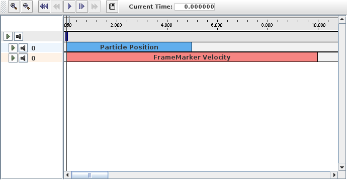
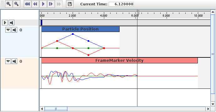
5.4.4 Data file format
The data files associated with numeric probes are ASCII files containing two lines of header information followed by a set of knot points, one per line, defining the numeric data. The time value (relative to the probe’s start time) for each knot point can be specified explicitly at the start of the each line, in which case the file takes the following format:
Knot point information begins on line 3, with each line being a
sequence of numbers giving the knot’s time followed by ![]() values,
where
values,
where ![]() is the vector size of the probe (i.e., the value returned by
getVsize()).
is the vector size of the probe (i.e., the value returned by
getVsize()).
Alternatively, time values can be implicitly specified starting at 0 (relative to the probe’s start time) and incrementing by a uniform timeStep, in which case the file assumes a second format:
For both formats, startTime, startTime, and scale are numbers giving the probe’s start and stop time in seconds and scale gives the scale factor (which is typically 1.0). interpolation is a word describing how the data should be interpolated between knot points and is the string value of Interpolation.Order as described in Section 5.4.1 (and which is typically Linear, Parabolic, or Cubic). vsize is an integer giving the probe’s vector size.
The last entry on the second line is either a number specifying a (uniform) time step for the knot points, in which case the file assumes the second format, or the keyword explicit, in which case the file assumes the first format.
As an example, the file used to specify data for the input probe in the example of Section 5.4.3 looks like the following:
Since the data is uniformly spaced beginning at 0, it would also be possible to specify this using the second file format:
5.4.5 Adding probe data in-line
It is also possible to specify input probe data directly in code, instead of reading it from a file. For this, one would use the constructor
which creates a NumericInputProbe with the specified property and with start and stop times indicated by t0 and t1. Data can then be added to this probe using the method
where data is an array of knot point data. This contains the
same knot point information as provided by a file (Section
5.4.4), arranged in row-major order. Times values
for the knots are either implicitly specified, starting at 0 (relative
to the probe’s start time) and increasing uniformly by the amount
specified by timeStep, or are explicitly specified at the
beginning of each knot if timeStep is set to the built-in
constant NumericInputProbe.EXPLICIT_TIME. The size of the data array should then be either ![]() (implicit time values) or
(implicit time values) or
![]() (explicit time values), where
(explicit time values), where ![]() is the probe’s vector size
and
is the probe’s vector size
and ![]() is the number of knots.
is the number of knots.
As an example, the data for the input probe in Section 5.4.3 could have been specified using the following code:
When specifying data in code, the interpolation defaults to Linear unless explicitly specified using setInterpolationOrder(), as in, for example:
5.4.6 Numeric monitor probes
In some cases, it may be useful for an application to deploy an output probe in which the data, instead of being collected from various component properties, is generated by a function within the probe itself. This ability is provided by a NumericMonitorProbe, which generates data using its generateData(vec,t,trel) method. This evaluates a vector-valued function of time at either the absolute time t or the probe-relative time trel and stores the result in the vector vec, whose size equals the vector size of the probe (as returned by getVsize()). The probe-relative time trel is determined by
| (5.1) |
where tstart and scale are the probe’s start time and scale factors as returned by getStartTime() and getScale().
As described further below, applications have several ways to control how a NumericMonitorProbe creates data:
-
•
Provide the probe with a DataFunction using the setDataFunction(func) method;
-
•
Override the generateData(vec,t,trel) method;
-
•
Override the apply(t) method.
The application is free to generate data in any desired way, and so in this sense a NumericMonitorProbe can be used similarly to a Monitor, with one of the main differences being that the data generated by a NumericMonitorProbe can be automatically displayed in the ArtiSynth GUI or written to a file.
The DataFunction interface declares an eval() method,
void eval (VectorNd vec, double t, double trel)
that for NumericMonitorProbes evaluates a vector-valued function of time, where the arguments take the same role as for the monitor’s generateData() method. Applications can declare an appropriate DataFunction and set or query it within the probe using the methods
The default implementation generateData() checks to see if a data function has been specified, and if so, uses that to generate the probe data. Otherwise, if the probe’s data function is null, the data is simply set to zero.
To create a NumericMonitorProbe using a supplied DataFunction, an application will create a generic probe instance, using one of its constructors such as
and then define and instantiate a DataFunction and pass it to the probe using setDataFunction(). It is not necessary to supply a file name (i.e., fileName can be null), but if one is provided, then the probe’s data can be saved to that file.
A complete example of this is defined in
artisynth.demos.tutorial.SinCosMonitorProbe
the listing for which is:
In this example, the DataFunction is implemented using the class SinCosFunction, which also implements Clonable and the associated clone() method. This means that the resulting probe will also be duplicatable within the GUI. Alternatively, one could implement SinCosFunction by extending DataFunctionBase, which implements Clonable by default. Probes containing DataFunctions which are not Clonable will not be duplicatable.
When the example is run, the resulting probe output is shown in the timeline image of Figure 5.5.
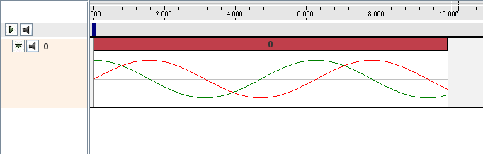
As an alternative to supplying a DataFunction to a generic NumericMonitorProbe, an application can instead subclass NumericMonitorProbe and override either its generateData(vec,t,trel) or apply(t) methods. As an example of the former, one could create a subclass as follows:
Note that when subclassing, one must also create constructor(s) for that subclass. Also, NumericMonitorProbes which don’t have a DataFunction set are considered to be clonable by default, which means that the clone() method may also need to be overridden if cloning requires any special handling.
5.4.7 Numeric control probes
In other cases, it may be useful for an application to deploy an input probe which takes numeric data, and instead of using it to modify various component properties, instead calls an internal method to directly modify the simulation in any way desired. This ability is provided by a NumericControlProbe, which applies its numeric data using its applyData(vec,t,trel) method. This receives the numeric input data via the vector vec and uses it to modify the simulation for either the absolute time t or probe-relative time trel. The size of vec equals the vector size of the probe (as returned by getVsize()), and the probe-relative time trel is determined as described in Section 5.4.6.
A NumericControlProbe is the Controller equivalent of a NumericMonitorProbe, as described in Section 5.4.6. Applications have several ways to control how they apply their data:
-
•
Provide the probe with a DataFunction using the setDataFunction(func) method;
-
•
Override the applyData(vec,t,trel) method;
-
•
Override the apply(t) method.
The application is free to apply data in any desired way, and so in this sense a NumericControlProbe can be used similarly to a Controller, with one of the main differences being that the numeric data used can be automatically displayed in the ArtiSynth GUI or read from a file.
The DataFunction interface declares an eval() method,
void eval (VectorNd vec, double t, double trel)
that for NumericControlProbes applies the numeric data, where the arguments take the same role as for the monitor’s applyData() method. Applications can declare an appropriate DataFunction and set or query it within the probe using the methods
The default implementation applyData() checks to see if a data function has been specified, and if so, uses that to apply the probe data. Otherwise, if the probe’s data function is null, the data is simply ignored and the probe does nothing.
To create a NumericControlProbe using a supplied DataFunction, an application will create a generic probe instance, using one of its constructors such as
and then define and instantiate a DataFunction and pass it to the probe using setDataFunction(). The latter constructor creates the probe and reads in both the data and timing information from the specified file.
A complete example of this is defined in
artisynth.demos.tutorial.SpinControlProbe
the listing for which is:
This example creates a simple box and then uses a NumericControlProbe to spin it about the ![]() axis, using a DataFunction implementation called SpinFunction. A clone method
is also implemented to ensure that the probe will be duplicatable in
the GUI, as described in Section 5.4.6. A
single channel of data is used to control the orientation angle of the
box about
axis, using a DataFunction implementation called SpinFunction. A clone method
is also implemented to ensure that the probe will be duplicatable in
the GUI, as described in Section 5.4.6. A
single channel of data is used to control the orientation angle of the
box about ![]() , as shown in Figure 5.6.
, as shown in Figure 5.6.
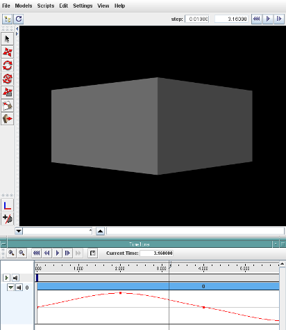
Alternatively, an application can subclass NumericControlProbe and override either its applyData(vec,t,trel) or apply(t) methods, as described for NumericMonitorProbes (Section 5.4.6).
5.5 Application-Defined Menu Items
Application models can define custom menu items that appear under the Application menu in the main ArtiSynth menu bar.
This can be done by implementing the interface HasMenuItems in either the RootModel or any of its top-level components (e.g., models, controllers, probes, etc.). The interface contains a single method
which, if the component has menu items to add, should append them to items and return true.
The RootModel and all models derived from ModelBase implement HasMenuItems by default, but with getMenuItems() returning false. Models wishing to add menu items should override this default declaration. Other component types, such as controllers, need to explicitly implement HasMenuItems.
Note: the Application menu will only appear if getMenuItems() returns true for either the RootModel or one or more of its top-level components.
getMenuItems() will be called each time the Application menu is selected, so the menu itself is created on demand and can be varied to suite the current system state. In general, it should return items that are capable of being displayed inside a Swing JMenu; other items will be ignored. The most typical item is a Swing JMenuItem. The convenience method createMenuItem(listener,text,toolTip) can be used to quickly create menu items, as in the following code segment:
This creates three menu items, each with this specified as an ActionListener and no tool-tip text, and appends them to items. They will then appear under the Application menu as shown in Figure 5.7.
To actually execute the menu commands, the items returned by getMenuItems() need to be associated with an ActionListener (defined in java.awt.event), which supplies the method actionPerformed() which is called when the menu item is selected. Typically the ActionListener is the component implementing HasMenuItems, as was assumed in the example declaration of getMenuItems() shown above. RootModel and other models derived from ModelBase implement ActionListener by default, with an empty declaration of actionPerformed() that should be overridden as required. A declaration of actionPerformed() capable of handling the menu example above might look like this:
Chapter 6 Finite Element Models
This section details how to construct three-dimensional finite element models, and how to couple them with the other simulation components described in previous sections (e.g. particles and rigid bodies). Finite element muscles, which have additional properties that allow them to contract given activation signals, are discussed in Section 6.8. An example FEM model of the masseter, coupled to a rigid jaw and maxilla, is shown in Figure 6.1.
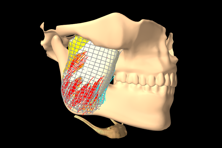
6.1 Overview
The finite element method (FEM) is a numerical technique used for solving a system of partial differential equations (PDEs) over some domain. The general approach is to divide the domain into a set of building blocks, referred to as elements. These partition the space, and form local domains over which the system of equations can be locally approximated. The corners of these elements, the nodes, become control points in a discretized system. The solution is then assumed to be smoothly interpolated across the elements based on values determined at the nodes. Using this discretization, the differential system is converted into an algebraic one, which is often linearized and solved iteratively.
In ArtiSynth, the PDEs considered are the governing equations of continuum mechanics: the conservation of mass, momentum, and energy. To complete the system, a constitutive equation is required that describes the stress-strain response of the material. This constitutive equation is what distinguishes between material types. The domain is the three-dimensional space that the model occupies. This must be divided into small elements which accurately represent the geometry. Within each element, the PDEs are sampled at a set of points, referred to as integration points, and terms are numerically integrated to form an algebraic system to solve.
The purpose of the rest of this section is to describe the construction and use of finite elements models within ArtiSynth. It does not further discuss the mathematical framework or theory. For an in-depth coverage of the nonlinear finite element method, as applied to continuum mechanics, the reader is referred to the textbook by Bonet and Wood [3].
6.1.1 FemModel3d
The basic type of finite element model is implemented in the class FemModel3d. This class controls some properties that are used by the model as a whole. The key ones that affect simulation dynamics are:
| Property | Description |
|---|---|
| density | The density of the model |
| material | An object that describes the material’s constitutive law (i.e. its stress-strain relationship). |
| particleDamping | Proportional damping associated with the particle-like motion of the FEM nodes. |
| stiffnessDamping | Proportional damping associated with the system’s stiffness term. |
These properties can be set and retrieved using the methods
Keep in mind that ArtiSynth is essentially ``unitless'' (Section 4.2), so it is the responsibility of the developer to ensure that all properties are specified in a compatible way.
The density of the model is used to compute the mass distribution throughout the volume. Note that we use a diagonally lumped mass matrix (DLMM) formulation, so the mass is assumed to be concentrated at the location of the discretized FEM nodes. To allow for a spatially-varying density, a mass can later be specified for each node individually.
The FEM’s material is a delegate object used to compute stress and stiffness within individual elements. It handles the constitutive component of the model. Materials will be discussed in more detail in Section 6.1.3.
The two damping parameters are related to Rayleigh damping, which is used to dissipate energy within finite element models. There are two proportional damping terms: one related to the system’s mass, and one related to stiffness. The resulting damping force applied is
| (6.1) |
where ![]() is the value of particleDamping,
is the value of particleDamping, ![]() is the value of
stiffnessDamping,
is the value of
stiffnessDamping, ![]() is the FEM model’s lumped mass matrix,
is the FEM model’s lumped mass matrix, ![]() is
the FEM’s stiffness matrix, and
is
the FEM’s stiffness matrix, and ![]() is the concatenated vector of FEM node
velocities. Since the lumped mass matrix is diagonal, the mass-related
component of damping can be applied separately to each FEM node. Thus, the
mass component reduces to the same system as Equation (3.3),
which is why it is referred to as ``particle damping''.
is the concatenated vector of FEM node
velocities. Since the lumped mass matrix is diagonal, the mass-related
component of damping can be applied separately to each FEM node. Thus, the
mass component reduces to the same system as Equation (3.3),
which is why it is referred to as ``particle damping''.
6.1.2 Component Structure
Each FemModel3d contains three lists of sub-components:
- nodes
-
The particle-like dynamic components of the model. These lie at the corners of the elements and carry all the mass (due to DLMM formulation).
- elements
-
The spatial building blocks of the model. These define the sub-units over which the system is numerically integrated.
- meshes
-
The geometry in the model. This includes the surface mesh, and any other embedded geometries.
An example showing each of these components is shown in Figure 6.2.
 |
 |
 |
 |
| (a) FEM model | (b) Nodes | (c) Elements | (d) Geometry |
Nodes
The set of nodes belong to a finite element model can be obtained by the method
Nodes are implemented in the class FemNode3d, which is a subclass of Particle (Section 3.1). They are the main dynamic components of the finite element model. The key properties affecting simulation dynamics are:
| Property | Description |
|---|---|
| restPosition | The initial position of the node. |
| position | The current position of the node. |
| velocity | The current velocity of the node. |
| mass | The mass of the node. |
| dynamic | Whether the node is considered dynamic or parametric (e.g. boundary condition). |
Each of these properties has corresponding getXxx() and setXxx(...) functions to access and modify them.
The restPosition property defines the node’s position in the FEM model’s ``natural'' or ``undeformed'' state. Rest positions are used to compute an initial configuration for the model, from which strains are determined. A node’s rest position can be updated in code using the method: FemNode3d.setRestPosition(Point3d).
If any node’s rest positions are changed, the current values for stress and stiffness will become invalid. They can be manually updated using the method FemModel3d.updateStressAndStiffness() for the parent model. Otherwise, stress and stiffness will be automatically updated at the beginning of the next time step.
The properties position and velocity give the node’s current 3D state. These are common to all point-like particles, as is the mass property. Here, however, mass represents the lumped mass of the immediately surrounding material. Its value is initialized by equally dividing mass contributions from each adjacent element, given their densities. For a finer control of spatially-varying density, node masses can be set manually after FEM creation.
The FEM node’s dynamic property specifies whether or not the node is considered when computing the dynamics of the system. If not, it is treated as being parametrically controlled. This has implications when setting boundary conditions (Section 6.1.4).
Elements
Elements are the spatial building blocks of the domain. Within each element, the displacement (or strain) field is interpolated from displacements at nodes:
 |
(6.2) |
where ![]() is the displacement of the
is the displacement of the ![]() th node that is adjacent to the
element, and
th node that is adjacent to the
element, and ![]() is referred to as the shape function (or
basis function) associated with that node. Elements are classified by
their shape, number of nodes, and shape function order (Table
6.1). ArtiSynth supports the following element types:
is referred to as the shape function (or
basis function) associated with that node. Elements are classified by
their shape, number of nodes, and shape function order (Table
6.1). ArtiSynth supports the following element types:
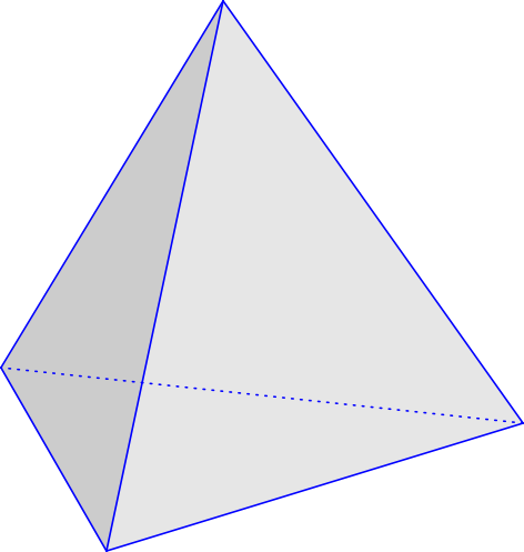 |
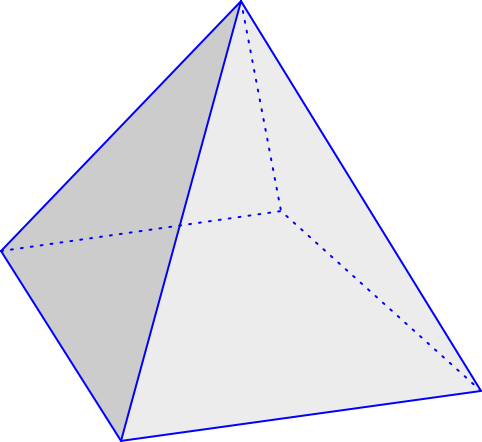 |
 |
 |
| TetElement, | PyramidElement, | WedgeElement, | HexElement, |
| QuadtetElement | QuadpyramidElement | QuadwedgeElement | QuadhexElement |
| Element Type | # Nodes | Order | # Integration Points |
|---|---|---|---|
| TetElement | 4 | linear | 1 |
| PyramidElement | 5 | linear | 5 |
| WedgeElement | 6 | linear | 6 |
| HexElement | 8 | linear | 8 |
| QuadtetElement | 10 | quadratic | 4 |
| QuadpyramidElement | 13 | quadratic | 5 |
| QuadwedgeElement | 15 | quadratic | 9 |
| QuadhexElement | 20 | quadratic | 14 |
The base class for all of these is FemElement3d. A numerical integration is performed within each element to create the (tangent) stiffness matrix. This integration is performed by evaluating the stress and stiffness at a set of integration points within each element, and applying numerical quadrature. The list of elements in a model can be obtained with the method
All objects of type FemModel3d have the following properties:
| Property | Description |
|---|---|
| density | Density of the element |
| material | An object that describes the constitutive law within the element (i.e. its stress-strain relationship). |
If left unspecified, the element’s density is inherited from the containing FemModel3d object. When set, the mass of the element is computed and divided amongst all its nodes, updating the lumped mass matrix.
Each element’s’ material property is also inherited by default from the containing FemModel3d. Specifying a material here allows for spatially-varying material properties across the model. Materials will be discussed further in Section 6.1.3.
Meshes
The geometry associated with a finite element model consists of a collection of meshes (e.g. PolygonalMesh, PolylineMesh, PointMesh) that move along with the model in a way that maintains the shape function interpolation equation (6.2) at each vertex location. These geometries can be used for visualizations, or for physical interactions like collisions. However, they have no physical properties themselves. FEM geometries will be discussed in more detail in Section 6.3. The list of meshes can be obtained with the method
6.1.3 Materials
The stress-strain relationship within each element is defined by a ``material'' delegate object, implemented by a subclass of FemMaterial. This material object is responsible for implementing the functions:
Inputs include a deformation gradient, pressure, and a coordinate frame that specifies potential directions of anisotropy. The default material type is LinearMaterial, where stress is related to strain through:
| (6.3) | |||
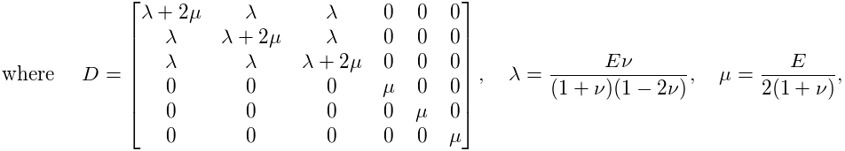 |
![]() is the standard
is the standard ![]() stress vector,
stress vector, ![]() is the
strain vector,
is the
strain vector, ![]() is the Young’s Modulus, and
is the Young’s Modulus, and ![]() is Poisson’s ratio. This
linear material uses a corotational formulation, so rotations are removed
per element before computing the strain [6]. To enable or
disable this corotational formulation, use
LinearMaterial.setCorotated(boolean).
is Poisson’s ratio. This
linear material uses a corotational formulation, so rotations are removed
per element before computing the strain [6]. To enable or
disable this corotational formulation, use
LinearMaterial.setCorotated(boolean).
All material models, including linear and non-linear, are available in the package artisynth.core.materials. A list of common materials is provided in Table 6.2. Those that are subclasses of IncompressibleMaterial allow for incompressibility.
| Material | Parameters | |
|---|---|---|
| LinearMaterial | Young’s modulus | |
| Poisson’s ratio | ||
| corotated | corotational formulation | |
| StVenantKirchoffMaterial | Young’s modulus | |
| Poisson’s ratio | ||
| NeoHookeanMaterial | Young’s modulus | |
| Poisson’s ratio | ||
| IncompNeoHookeanMaterial | shear modulus | |
| bulk modulus | ||
| MooneyRivlinMaterial | distortional parameters | |
| bulk modulus | ||
| OgdenMaterial | material parameters | |
| bulk modulus |
6.1.4 Boundary conditions
Boundary conditions can be implemented in one of several ways:
-
1.
Explicitly setting FEM node positions/velocities
-
2.
Attaching FEM nodes to other dynamic components
-
3.
Enabling collisions
To enforce an explicit (Dirichlet) boundary condition for a set of nodes, their dynamic property must be set to false. This notifies ArtiSynth that the state of these nodes (both position and velocity) will be controlled parametrically. By disabling dynamics, a fixed boundary condition is applied. For a moving boundary, positions and velocities of the boundary nodes must be explicitly set every timestep. This can be accomplished with either a Controller (see Section 5.3) or an InputProbe (see Section 5.4). Note that both the position and velocity of the nodes should be explicitly set for consistency.
Another type of supported boundary condition is to attach FEM nodes to other components, including particles, springs, rigid bodies, and locations within other FEM elements. Here, the node is still considered dynamic, but its motion is coupled to that of the attached component through a constraint mechanism. Attachments will be discussed further in Section 6.4.
Finally, the boundary of a FEM can be constrained by enabling collisions with other components. This will be covered in Section 6.9.
6.2 FEM model creation
Creating a finite element model in ArtiSynth typically follows the pattern:
The main code block for the FEM setup should do the following:
-
•
Build the node/element structure
-
•
Set physical properties
-
–
density
-
–
damping
-
–
material
-
–
-
•
Set boundary conditions
-
•
Set render properties
Building the FEM structure can be done with the use of factory methods for simple shapes, by loading external files, or by writing code to manually assemble the nodes and elements.
6.2.1 Factory methods
For simple shapes such as beams and ellipsoids, there are factory methods to automatically build the node and element structure. These methods are found in the FemFactory class. Some common methods are
The inputs specify the dimensions, resolution, and potentially the type of element to use. The following code creates a basic beam made up of hexahedral elements:
6.2.2 Loading external FEM meshes
For more complex geometries, volumetric meshes can be loaded from external files. A list of supported file types is provided in Table 6.3. To load a geometry, an appropriate file reader must be created. Readers capable of reading FEM models implement the interface FemReader, which has the method
Additionally, many FemReader classes have static methods to handle the loading of files for convenience.
| Format | File extensions | Reader | Writer |
|---|---|---|---|
| ANSYS | .node, .elem | AnsysReader | AnsysWriter |
| TetGen | .node, .ele | TetGenReader | TetGenWriter |
| Abaqus | .inp | AbaqusReader | AbaqusWriter |
| VTK (ASCII) | .vtk | VtkAsciiReader | – |
The following code snippet demonstrates how to load a model using the AnsysReader.
The method ArtisynthPath.getSrcRelativePath() is used to find a path within the ArtiSynth source tree that is relative to the current model’s source file. Note the try-catch block. Most of these readers throw an IOException if the read fails.
6.2.3 Generating from surfaces
There are two ways a FEM model can be generated from a surface: by using a FEM mesh generator, and by extruding a surface along its normal direction.
ArtiSynth has the ability to interface directly with the TetGen library (http://tetgen.org) to create a tetrahedral volumetric mesh given a closed and manifold surface. The main Java class for calling TetGen directly is TetgenTessellator. The tessellator has several advanced options, allowing for the computation of convex hulls, and for adding points to a volumetric mesh. For simply creating a FEM from a surface, there is a convenience routine within FemFactory that handles both mesh generation and constructing a FemModel3d:
If quality ![]() , then points will be added in an attempt to bound the
maximum radius-edge ratio (see the -q switch for TetGen). According
to the TetGen documentation, the algorithm usually succeeds for a
quality ratio of 1.2.
, then points will be added in an attempt to bound the
maximum radius-edge ratio (see the -q switch for TetGen). According
to the TetGen documentation, the algorithm usually succeeds for a
quality ratio of 1.2.
It’s also possible to create thin layer of elements by extruding a surface along its normal direction.
For example, to create a two-layer slice of elements centered about a surface of a tendon mesh, one might use
For this type of extrusion, triangular faces become wedge elements, and quadrilateral faces become hexahedral elements.
Note: for extrusions, no care is taken to ensure element quality; if the surface has a high curvature relative to the total extrusion thickness, then some elements will be inverted.
6.2.4 Building elements in code
A finite element model’s structure can also be manually constructed in code. FemModel3d has the methods:
For an element to successfully be added, all its nodes must already have been added to the model. Nodes can be constructed from a 3D location, and elements from an array of nodes. A convenience routine is available in FemElement3d that automatically creates the appropriate element type given the number of nodes (Table 6.1):
Be aware of node orderings when supplying nodes. For linear elements, ArtiSynth uses a clockwise convention with respect to the outward normal for the first face, followed by the opposite node(s). To determine the correct ordering for a particular element, check the coordinates returned by the function FemElement3d.getNodeCoords(). This returns the concatenated coordinate list for an ``ideal'' element of the given type.
6.2.5 Example: a simple beam model
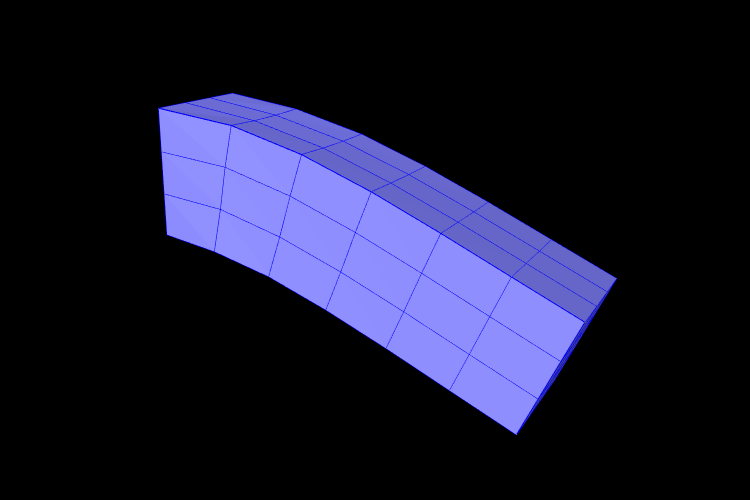
A complete application model that implements a simple FEM beam is given below.
This example can be found in artisynth.demos.tutorial.FemBeam. The build() method first creates a MechModel and FemModel3d. A FEM beam is created using a factory method on line 36. This beam is centered at the origin, so its length extends from -length/2 to length/2. The density, damping and material properties are then assigned.
On lines 45–49, a fixed boundary condition is set to the left-hand side of the beam by setting the corresponding nodes to be non-dynamic. Due to numerical precision, a small EPSILON buffer is required to ensure all left-hand boundary nodes are identified (line 46).
Rendering properties are then assigned to the FEM model on line 52. These will be discussed further in Section 6.10.
6.3 FEM Geometry
Associated with each FEM model is a list of geometry with the heading meshes. This geometry can be used for either display purposes, or for interactions such as collisions. A geometry itself has no physical properties; its motion is entirely governed by the FEM model that contains it.
All FEM geometries are of type FemMeshComp, which stores a reference to a mesh object (Section 2.5), as well as attachment information that links vertices of the mesh to points within the FEM. The attachments enforce the shape function interpolation in Equation (6.2) to hold at each mesh vertex, with constant shape function coefficients.
6.3.1 Surface meshes
By default, every FemModel3d has an auto-generated geometry representing the ``surface mesh''. The surface mesh consists of all un-shared element faces (i.e. the faces of individual elements that are exposed to the world), and its vertices correspond to the nodes that make up those faces. As the FEM nodes move, so do the mesh vertices due to the attachment framework.
The surface mesh can be obtained using one of the following functions in FemModel3d:
The first returns the surface complete with attachment information. The latter method directly returns the PolygonalMesh that is controlled by the FEM.
It is possible to manually set the surface mesh:
However, doing so is normally not necessary. It is always possible to add additional mesh geometries to a finite element model, and the visibility settings can be changed so that the default surface mesh is not rendered.
6.3.2 Embedding geometry within an FEM
Any geometry of type MeshBase can be added to a FemModel3d. To do so, first position the mesh so that its vertices are in the desired locations inside the FEM, then call one of the FemModel3d methods:
The latter is a convenience routine that also gives the newly embedded FemMeshComp a name.
6.3.3 Example: a beam with an embedded sphere
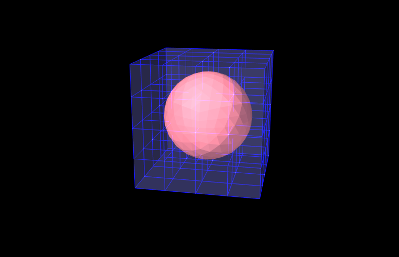
A complete model demonstrating embedding a mesh is given below.
This example can be found in artisynth.demos.tutorial.FemEmbeddedSphere. The model is very similar to FemBeam. A MechModel and FemModel3d are created and added. At line 41, a PolygonalMesh of a sphere is created using a factory method. The sphere is already centered inside the beam, so it does not need to be repositioned. At Line 42, the sphere is embedded inside model fem, creating a FemMeshComp with the name ``sphere''. The full model is shown in Figure 6.4.
6.4 Node attachments
To couple FEM models to other dynamic components, the ``attachment'' mechanism described in Section 1.2 is used. This involves creating and adding to the model attachment components, which are instances of DynamicAttachment, as described in Section 3.5. Common point-based attachment classes are listed in Table 6.4.
| Attachment | Description |
|---|---|
| PointParticleAttachment | Attaches one ``point'' to one ``particle'' |
| PointFrameAttachment | Attaches one ``point'' to one ``frame'' |
| PointFem3dAttachment | Attaches one ``point'' to a linear combination of FEM nodes |
FEM models are connected to other model components by attaching their nodes to various components. This can be done by creating an attachment object of the appropriate type, and then adding it to the MechModel using
There are also convenience routines inside MechModel that will create the appropriate attachments automatically (see Section 3.5.1).
6.4.1 Connecting nodes to rigid bodies or particles
Since FemNode3d is a subclass of Particle, the same methods described in Section 3.5.1 for attaching particles to other particles and frames are available. For example, we can attach an FEM node to a rigid body using a either a statement of the form
or the following equivalent statement which does the same thing:
Both of these create a PointFrameAttachment between a rigid body (called body) and an FEM node (called node) and then adds it to the MechModel mech.
6.4.2 Example: connecting a beam to a block
The following model demonstrates attaching a FEM beam to a rigid block.
This model extends the FemBeam example of Section 6.2.5. The build() method then creates and adds a RigidBody block (lines 18–20). On line 21, the block is repositioned to the side of the beam to prepare for the attachment. On lines 24–28, all right-most nodes of the beam are then set to be attached to the block using a PointFrameAttachment. In this case, the attachments are explicitly created. They could also have been attached using
6.4.3 Connecting nodes directly to elements
Typically, nodes do not align in a way that makes it
possible to connect them to other FEM models and/or points based on
simple point-to-node attachments. Instead, we use a different
mechanism that allows us to attach a point to an arbitrary location
within a FEM model. This is done using an attachment component of
type
PointFem3dAttachment, which
implements an attachment where the position ![]() and velocity
and velocity ![]() of the
attached point is determined by a weighted sum of the positions
of the
attached point is determined by a weighted sum of the positions ![]() and velocities
and velocities ![]() of selected fem nodes:
of selected fem nodes:
| (6.4) |
Any force ![]() acting on the attached point is then propagated back
to the nodes, according to the relation
acting on the attached point is then propagated back
to the nodes, according to the relation
| (6.5) |
where ![]() is the force acting on node
is the force acting on node ![]() due to
due to ![]() . This
relation can be derived based on the conservation of energy.
If
. This
relation can be derived based on the conservation of energy.
If ![]() is embedded within a single element, then the
is embedded within a single element, then the ![]() are
simply the element nodes and the
are
simply the element nodes and the ![]() are corresponding shape
function values; this is known as an element-based attachment.
On the other hand, as desribed below, it is sometimes desirable to
form an attachment using a more general set of nodes that extends
beyond a single element; this is known as a nodal-based
attachment (Section 6.4.5).
are corresponding shape
function values; this is known as an element-based attachment.
On the other hand, as desribed below, it is sometimes desirable to
form an attachment using a more general set of nodes that extends
beyond a single element; this is known as a nodal-based
attachment (Section 6.4.5).
An element-based attachment can be created using a code fragment of the form
First, a PointFem3dAttachment is created for the point pnt. Next, setFromElement() is used to determine the nodal weights within the element elem for the specified position (which in this case is simply the point’s current position). To do this, it computes the ``natural coordinates'' coordinates of the position within the element. For this to be guaranteed to work, the position should be on or inside the element. If natural coordinates cannot be found, the method will return false and the nearest estimates coordinates will be used instead. However, it is sometimes possible to find natural coordinates outside a given element as long as the shape functions are well-defined. Finally, the attachment is added to the model.
More conveniently, the exact same functionality is provided by the attachPoint() method in MechModel:
This creates an attachment identical to that created by the previous code fragment.
Often, one does not want to have to determine the element to which a point should be attached. In that case, one can call
or, equivalently,
This will find the nearest element to the node in question and use that to create the attachment. If the node is outside the FEM model, then it will be attached to the nearest point on the FEM’s surface.
6.4.4 Example: connecting two FEMs together
The following model demonstrates how to attach two FEM models together:
This example can be found in artisynth.demos.tutorial.FemBeamWithFemSphere. The model extends FemBeam, adding a finite element sphere and coupling them together. The sphere is created and added on lines 18–28. It is read from TetGen-generated files using the TetGenReader class. The model is then scaled to match the dimensions of the current model, and transformed to the right side of the beam. To create attachments, the code first checks for any nodes that belong to the sphere that fall inside the beam using the FemModel3d.findContainingElement(Point3d) method (line 36), which returns the containing element if the point is inside the model, or null if the point is outside. Internally, this spatial search uses a bounding volume hierarchy for efficiency (see BVTree and BVFeatureQuery). If the point is contained within the beam, then mech.attachPoint() is used to attach it to the nodes of the element (line 39).
6.4.5 Nodal-based attachments
The example of Section 6.4.4 uses element-based attachments to connect the nodes of one FEM to elements of another. As mentioned above, element-based attachments assume that the attached point is associated with a specific FEM model element. While this often gives good results, there are situations where it may be desirable to distribute the connection more broadly among a larger set of nodes.
In particular, this is sometimes the case when connecting FEM models to point-to-point springs. The end-point of such a spring may end up exerting a large force on the FEM, and then if the number of nodes to which the end-point is attached are too small, the resulting forces on these nodes (Equation 6.5) may end up being too large. In other words, it may be desirable to distribute the spring’s force more evenly throughout the FEM model.
To handle such situations, it is possible to create a nodal-based attachment in which the nodes and weights are explicitly specified. This involves explicitly creating a PointFem3dAttachment for the point or particle to be attached and the specifying the nodes and weights directly,
where nodes and weights are arrays of FemNode and double, respectively. It is up to the application to determine these.
PointFem3dAttachment provides several methods for explicitly specifying nodes and weights. The signatures for these include:
The last two methods determine the weights automatically, using an
inverse-distance-based calculation in which each weight ![]() is initially computed as
is initially computed as
 |
(6.6) |
where ![]() is the distance from node
is the distance from node ![]() to pos and
to pos and
![]() is the maximum distance. The weights are then
adjusted to ensure that they sum to one and that the weighted sum of
the nodes equals pos. In some cases, the specified nodes
may not provide enough support for the last condition to be
met, in which case the methods return false.
is the maximum distance. The weights are then
adjusted to ensure that they sum to one and that the weighted sum of
the nodes equals pos. In some cases, the specified nodes
may not provide enough support for the last condition to be
met, in which case the methods return false.
6.4.6 Example: element vs. nodal-based attachments
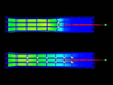
The model demonstrating the difference between element and nodal-based attachments is defined in
artisynth.demos.tutorial.PointFemAttachment
It creates two FEM models, each with a single point-to-point spring attached to a particle at their center. The model at the top (fem1 in the code below) is connected to the particle using an element-based attachment, while the lower model (fem2 in the code) is connected using a nodal-based attachment with a larger number of nodes. Figure 6.7 shows the result after the model is run until stable. The element-based attachment results in significantly higher deformation in the immediate vicinity around the attachment, while for the nodal-based attachment, the deformation is distributed much more evenly through the model.
The build method and some of the auxiliary code for this model is shown below. Code for the other auxiliary methods, including addFem(), addParticle(), addSpring(), and setAttachedNodesWhite(), can be found in the actual source file.
The build() method begins by creating a MechModel and then adding to it two FEM beams (created using the auxiliary method addFem(). Rendering of each FEM model’s surface is then set up to show strain values (setSurfaceRendering(), lines 41 and 43). The surface meshes themselves are also redefined to exclude the frontmost elements, allowing the strain values to be displayed closer model centers. This redefinition is done using calls to createSurfaceMesh() (lines 40, 41) with a custom ElementFilter defined at lines 3-12.
Next, the end-point particles for the axial springs are created (using the auxiliary method addParticle(), lines 46-49), and particle m1 is attached to fem1 using mech.attachPoint() (line 52), which creates an element-based attachment at the point’s current location. Point m2 is then attached to fem2 using a nodal-based attachment. The nodes for these are collected as the union of all nodes for a specufied set of elements (lines 58-59, and the method collectNodes() defined at lines 16-25). These are then used to create a nodal-based attachment (lines 61-63), where the weights are determined automatically using the method associated with equation (6.6).
Finally, the springs are created (auxiliary method addSpring(), lines 66-67), the nodes associated for each attachment are set to render as white spheres (setAttachedNodesWhites(), lines 70-71), and the particles are set to render as green spheres.
To run this example in ArtiSynth, select All demos > tutorial > PointFemAttachment from the Models menu. Running the model will cause it to settle into the state shown in Figure 6.7. Selecting and dragging one of the spring anchor points at the right will cause the spring tension to vary and further illustrate the difference between the element and nodal-based attachments.
6.5 FEM markers
Just as there are FrameMarkers to act as anchor points on a frame or rigid body (Section 3.2.1), there are also FemMarkers that can mark a point inside a finite element. They are frequently used to provide anchor points for attaching springs and forces to a point inside an element, but can also be used for graphical purposes.
FEM markers are implemented by the class FemMarker, which is a subclass of Point. They are essentially massless points that contain their own attachment component, so when creating and adding a marker there is no need to create a separate attachment component.
Within the component hierarchy, FEM markers are typically stored in the markers list of their associated FEM model. They can be created and added using a code fragment of the form
This creates a marker at the location ![]() (in world
coordinates), calls setFromFem() to attach it to the nearest
element in the FEM model ( which is either the containing element or
the nearest element on the model’s surface), and then adds it to the
markers list.
(in world
coordinates), calls setFromFem() to attach it to the nearest
element in the FEM model ( which is either the containing element or
the nearest element on the model’s surface), and then adds it to the
markers list.
If the marker’s attachment has not already been set when addMarker() is called, then addMarker() will call setFromFem() automatically. Therefore the above code fragment is equivalent to the following:
Alternatively, one may want to explicitly specify the nodes associated with the attachment, as described in Section 6.4.5:
There are a variety of methods available to set the attachment, mirroring those available in the underlying base class PointFem3dAttachment:
The last two methods compute nodal weights automatically, as described in Section 6.4.5, based on the marker’s currently assigned position. If the supplied nodes do not provide sufficient support, then the methods return false.
Another set of convenience methods are supplied by FemModel3d, which combine these with the addMarker() call:
For example, one can do
Markers are often used to track movement within an FEM model. For that, one can examine their positions and velocities, as with any other particles, using the methods
The return values from these methods should not be
modified. Alternatively, when a 3D force ![]() is applied to the
marker, it is distributed to the attached nodes according to the nodel
weights, as described in Equation (6.5).
is applied to the
marker, it is distributed to the attached nodes according to the nodel
weights, as described in Equation (6.5).
6.5.1 Example: attaching a FEM beam to a muscle
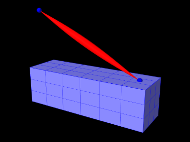
A complete application model that employs a fem marker as an anchor for a spring is given below.
This example can be found in artisynth.demos.tutorial.FemBeamWithMuscle. This model extends the FemBeam example, adding a FemMarker for the spring to attach to. The method createMarker(...) on lines 29–35 is used to create and add a marker to the FEM. Since the element is initially set to null, when it is added to the FEM, the model searches for the containing or nearest element. The loaded model is shown in Figure 6.8.
6.6 Frame attachments
It is also possible to attach frame components, including rigid bodies, directly to FEM models, using the attachment component FrameFem3dAttachment. Analagously to PointFem3dAttachment, the attachment is implemented by connecting the frame to a set of FEM nodes, and attachments can be either element-based or nodal-based. The frame’s origin is computed in the same way as for point attachments, using a weighted sum of node positions (Equation 6.4), while the orientation is computed using a polar decomposition on a deformation gradient determined from either element shape functions (for element-based attachments) or a Procrustes type analysis using nodal rest positions (for nodal-based attachments).
An element-based attachment can be created using either a code fragment of the form
or, equivalently, the attachFrame() method in MechModel:
This attaches the frame frame to the nodes of the FEM element elem. As with PointFem3dAttachment, if the frame’s origin is not inside the element, it may not be possible to accurately compute the internal nodal weights, in which case setFromElement() will return false.
In order to have the appropriate element located automatically, one can instead use
or, equivalently,
As with point-to-FEM attachments, it may be desirable to create a nodel-based attachment in which the nodes and weights are not tied to a specific element. The reasons for this are generally the same as with nodal-based point attachments (Section 6.4.5): the need to distribute the forces and moments acting on the frame across a broader set of element nodes. Also, element-based frame attachments use element shape functions to determine the frame’s orientation, which may produce slightly asymmetric results if the frame’s origin is located particularly close to a specific node.
FrameFem3dAttachment provides several methods for explicitly specifying nodes and weights. The signatures for these include:
Unlike their counterparts in PointFem3dAttachment, the first two methods also require the current desired pose of the frame TFW (in world coordinates). This is because while nodes and weights will unambiguously specify the frame’s origin, they do not specify the desired orientation.
6.6.1 Example: attaching frames to a FEM beam
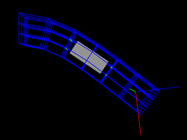
A model illustrating how to connect frames to a FEM model is defined in
artisynth.demos.tutorial.FrameFemAttachment
It creates a FEM beam, along with a rigid body block and a massless coordinate frame, that are then attached to the beam using nodal and element-based attachments. The build method is shown below:
Lines 3-22 create a MechModel and populate it with an FEM beam and a rigid body box. Next, a basic Frame is created, with a specified pose and an axis length of 0.3 (to allow it to be seen), and added to the MechModel (lines 25-28). It is then attached to the FEM beam using an element-based attachment (line 30). Meanwhile, the box is attached to using a nodal-based attachment, created from all the nodes associated with elements 22 and 31 (lines 33-36). Finally, all attachment nodes are set to be rendered as green spheres (lines 39-41).
To run this example in ArtiSynth, select All demos > tutorial > FrameFemAttachment from the Models menu. Running the model will cause it to settle into the state shown in Figure 6.9. Forces can interactively be applied to the attached block and frame using pull manipulator, causing the FEM model to deform (see the section ``Pull Manipulator'' in the ArtiSynth User Interface Guide).
6.6.2 Adding joints to FEM models
The ability to connect frames to FEM models, as described in Section 6.6, makes it possible to interconnect different FEM models directly using joints, as described in Section 3.3. This is done internally by using FrameFem3dAttachments to connect frames C and D of the joint (Figure 3.4) to their respective FEM models.
As indicated in Section 3.3.2, most joints have a constructor of the form
that creates a joint connecting bodyA to bodyB, with the initial pose of the D frame given (in world coordinates) by TDW. The same body and transform settings can be made on an existing joint using the method setBodies(bodyA, bodyB, TDW). For these constructors and methods, it is possible to specify FEM models for bodyA and/or bodyB. Internally, the joint then creates a FrameFem3dAttachment to connect frame C and/or D of the joint (See Figure 3.4) to the corresponding FEM model.
However, unlike joints involving rigid bodies or frames, there are no
associated ![]() or
or ![]() transforms (since there is no fixed
frame within an FEM to define such transforms). Methods or
constructors which utilize
transforms (since there is no fixed
frame within an FEM to define such transforms). Methods or
constructors which utilize ![]() or
or ![]() can therefore
not be used with FEM models.
can therefore
not be used with FEM models.
6.6.3 Example: two FEM beams connected by a joint
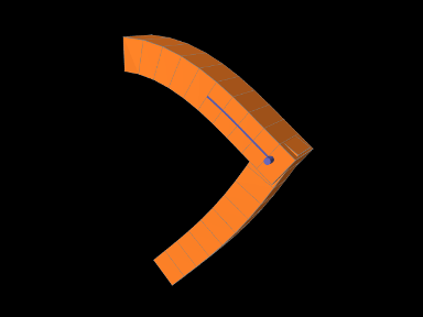
A model connecting two FEM beams by a joint is defined in
artisynth.demos.tutorial.JointedFemBeams
It creates two FEM beams and connects them via a special slotted-revolute joint. The build method is shown below:
Lines 3-16 create a MechModel and populates it with two FEM beams, fem1 and fem2, using an auxiliary method addFem() defined in the model source file. The leftmost nodes of fem1 are set fixed. A SlottedRevoluteJoint is then created to interconnect fem1 and fem2 at a location specified by TDW (lines 19-21). Lines 24-30 set some parameters for the joint, along with various render properties.
To run this example in ArtiSynth, select All demos > tutorial > JointedFemBeams from the Models menu. Running the model will cause it drop and flex under gravity, as shown in 6.10. Forces can interactively be applied to the beams using pull manipulator (see the section ``Pull Manipulator'' in the ArtiSynth User Interface Guide).
6.7 Incompressiblity
FEM incompressibility within ArtiSynth is enforced by trying to ensure that the volume of a FEM remains locally constant. This, in turn, is accomplished by constraining nodal velocities so that the local volume change, or divergence, is zero (or close to zero). There are generally two ways to do this:
-
•
Hard incompressibility, which sets up explicit constraints on the nodal velocities;
-
•
Soft incompressibility, which uses a restoring pressure based on a potential field to try to keep the volume constant.
Both of these methods operate independently, and both can be used either separately or together. Generally speaking, hard incompressibility will result in incompressibility being more rigorously enforced, but at the cost of increased computation time and (sometimes) less stability. Soft incompressibility allows the application to control the restoring force used to enforce incompressibility, usually by adjusting the value of the bulk modulus material property. As the bulk modulus is increased, soft incompressibility starts to act more like ‘hard’ incompressibility, with an infinite bulk modulus corresponding to perfect incompressibilty. However, very large bulk modulus values will generally produce stability problems.
6.7.1 Volume regions and locking
Both hard and soft incompressibility can be applied to different regions of local volume. From larger to smaller, these regions are:
-
•
Nodal - the local volume surrounding each node;
-
•
Element - the volume of each element;
-
•
Full - the volume at each integration point.
Element-based incompressibility is the standard method generally seen
in the literature. However, it tends not to work well for
tetrahedral meshes, because constraining the volume of each tet in a
tetrahedral mesh tends to over constrain the system. This is because
the number of tets in a large tetrahedral mesh is often ![]() ,
where
,
where ![]() is the number of nodes, and so putting a volume constraint
on each element may result in
is the number of nodes, and so putting a volume constraint
on each element may result in ![]() constraints, which exceeds the
constraints, which exceeds the
![]() degrees of freedom (DOF) in the FEM. This overconstraining results in an
artificially increased stiffness known as locking. Because of
locking, for tetrahedrally based meshes it may be better to use
nodal-based incomressibility, which creates a single volume constraint
around each node, resulting in only
degrees of freedom (DOF) in the FEM. This overconstraining results in an
artificially increased stiffness known as locking. Because of
locking, for tetrahedrally based meshes it may be better to use
nodal-based incomressibility, which creates a single volume constraint
around each node, resulting in only ![]() constraints, leaving
constraints, leaving ![]() DOF
to handle the remaining deformation. However, nodal-based
imcompressibility is computationally more costly than element-based
and may not be as stable.
DOF
to handle the remaining deformation. However, nodal-based
imcompressibility is computationally more costly than element-based
and may not be as stable.
Generally, the best solution for incompressible problems is to use
element-based incompressibility with a mesh consisting of hexahedra,
or primarily hexahedra and a mix of other elements (the latter
commonly being known as a hex dominant mesh). For hex-based
meshes, the number of elements is roughly equal to the number of
nodes, and so adding a volume constraint for each element imposes ![]() constraints on the model, which (like nodal incompressibility)
leaves
constraints on the model, which (like nodal incompressibility)
leaves ![]() DOF to handle the remaining deformation.
DOF to handle the remaining deformation.
Full incompressibility tries to control the volume at each integration point within each element, which almost always results in a large number of volumetric constraints and hence locking. It is therefore not commonly used and is provided mostly for debugging and diagnostic purposes.
6.7.2 Hard incompressibility
Hard incompressibility is controlled by the incompressible property of the FEM, which can be set to one of the following values of the enumerated type FemModel.IncompMethod:
- OFF
-
No hard incompressibility enforced.
- ELEMENT
-
Element-based hard incompressibility enforced (Section 6.7.1).
- NODAL
-
Nodal-based hard incompressibility enforced (Section 6.7.1).
- AUTO
-
Selects either ELEMENT or NODAL, with the former selected if the number of elements is less than or equal to the number of nodes.
- ON
-
Same as AUTO.
Hard incompressibility uses explicit constraints on the nodal velocities to enforce the incompressibilty, which increases computational cost. Also, if the number of constraints is too large, perturbed pivot errors may be encountered by the solver. However, hard incompressibility can in principle handle situtations where complete incompressibility is required. It is equivalent to the mixed u-P formulation used in commercial FEM codes (such as ANSYS), and the Lagrange multipliers computed for the constraints are pressure impulses.
Hard incompressibility can be applied in addition to soft incompressibility, in which case it will provide additional incompressibility enforcement on top of that provided by the latter. It can also be applied to linear materials, which are not themselves able to emulate true incompressible behavior (Section 6.7.4).
6.7.3 Soft incompressibility
Soft incompressibility enforces incompressibility using a restoring
pressure that is controlled by a volume-based energy potential. It is
only available for FEM materials that are subclasses of
IncompressibleMaterial.
The energy potential ![]() is a function of the determinant
is a function of the determinant ![]() of the
deformation gradient, and is scaled by the material’s bulk modulus
of the
deformation gradient, and is scaled by the material’s bulk modulus
![]() . The restoring pressure
. The restoring pressure ![]() is given by
is given by
 |
(6.7) |
Different potentials can be selected by setting the bulkPotential property of the incompressible material, whose value is an instance of IncompressibleMaterial.BulkPotential. Currently there are two different potentials:
- QUADRATIC
-
The potential and associated pressure are given by
(6.8) - LOGARITHMIC
-
The potential and associated pressure are given by
(6.9)
The default potential is QUADRATIC, which may provide slightly improved stability characteristics. However, we have not noticed significant differences between the two potentials in practice.
How soft incompressibility is applied within a FEM model is controlled by the FEM’s softIncompMethod property, which can be set to one of the following values of the enumerated type FemModel.IncompMethod:
- ELEMENT
-
Element-based soft incompressibility enforced (Section 6.7.1).
- NODAL
-
Nodal-based soft incompressibility enforced (Section 6.7.1).
- AUTO
-
Selects either ELEMENT or NODAL, with the former selected if the number of elements is less than or equal to the number of nodes.
- FULL
-
Incompressibility enforced at each integration point (Section 6.7.1).
6.7.4 Incompressibility and linear materials
Within a linear material, incompressibility is controlled by Poisson’s
ratio ![]() , which for isotropic materials can assume a value in the
range
, which for isotropic materials can assume a value in the
range ![]() . This specifies the amount of transvere contraction
(or expansion) exhibited by the material as it compressed or extended
along a particular direction. A value of
. This specifies the amount of transvere contraction
(or expansion) exhibited by the material as it compressed or extended
along a particular direction. A value of ![]() allows the material to be
compressed or extended without any transverse contraction or
expansion, while a value of
allows the material to be
compressed or extended without any transverse contraction or
expansion, while a value of ![]() in theory indicates a perfectly
incompressible material. However, setting
in theory indicates a perfectly
incompressible material. However, setting ![]() in practice
causes a division by zero, so only values close to 0.5 (such as 0.49)
can be used.
in practice
causes a division by zero, so only values close to 0.5 (such as 0.49)
can be used.
Moreover, the incompressibility only applies to small displacements,
so that even with ![]() it is still possible to squash a linear
FEM completely flat if enough force is applied. If true incompressible
behavior is desired with a linear material, then one must also use
hard incompressibility (Section 6.7.2).
it is still possible to squash a linear
FEM completely flat if enough force is applied. If true incompressible
behavior is desired with a linear material, then one must also use
hard incompressibility (Section 6.7.2).
6.7.5 Using incompressibility in practice
As mentioned above, when modeling incompressible models, we have found that the best practice is to use, if possible, either a hex or hex-dominant mesh, along with element-based incompressibility.
Hard incompressibility allows the handling of full incompressibility but at the expense of greater computational cost and often less stability. When modeling biomechanical materials, it is often permissible to use only soft incompressibility, partly since biomechanical materials are rarely completely incompressible. When implementing soft incompressibility, it is common practice to set the bulk modulus to something like 100 times the other (deviatoric) stiffnesses of the material.
We have found stability behavior to be complex, and while hard incompressibilty often results in less stable behavior, this is not always the case: in some situations the stronger enforcement afforded by hard incompressibility actually improves stabilty.
6.8 Muscle activated FEM models
Finite element muscle models are an extension to regular FEM models. As such, everything previously discussed for regular FEM models also applies to FEM muscles. Muscles have additional properties that allow them to contract when activated. There are two types of muscles supported:
- Fibre-based:
-
Point-to-point muscle fibres are embedded in the model.
- Material-based:
-
An auxiliary material is added to the constitutive law to embed muscle properties.
In this section, both types will be described.
6.8.1 FemMuscleModel
The main class for FEM-based muscles is FemMuscleModel, a subclass of FemModel3d. It differs from a basic FEM model in that it has the new property
| Property | Description |
| muscleMaterial | An object that adds an activation-dependent ‘muscle’ term to the constitutive law. |
This is a delegate object of type MuscleMaterial that computes activation-dependent stress and stiffness in the muscle. In addition to this property, FemMuscleModel adds two new lists of subcomponents:
- bundles
-
Groupings of muscle sub-units (fibres or elements) that can be activated. - exciters
-
Components that control the activation of a set of bundles or other exciters.
Bundles
Muscle bundles allow for a muscle to be partitioned into separate groupings of fibres/elements, where each bundle can be activated independently. They are implemented in the class MuscleBundle. Bundles have three key properties:
| Property | Description |
|---|---|
| excitation | Activation level of the muscle, |
| fibresActive | Enable/disable ``fibre-based'' muscle components. |
| muscleMaterial | An object that adds an activation-dependent ‘muscle’ term to the constitutive law. |
The excitation property controls the level of muscle activation, with zero being no muscle action, and one being fully activated. The fibresActive property is a boolean variable that controls whether or not to treat any contained fibres as point-to-point-like muscles (``fibre-based''). If false, the fibres are ignored. The third property, muscleMaterial, allows for a MuscleMaterial to be specified per bundle. By default, its value is inherited from FemMuscleModel.
Exciters
Muscle exciters enable you to simultaneously activate a group of ``excitation components''. This includes: point-to-point muscles, muscle bundles, muscle fibres, material-based muscle elements, and other muscle exciters. Components that can be excited all implement the ExcitationComponent interface. To add or remove a component to the exciter, use
If a gain factor is specified, the activation is scaled by the gain for that component.
6.8.2 Fibre-based muscles
In fibre-based muscles, a set of point-to-point muscle fibres are added between FEM nodes or markers. Each fibre is assigned an AxialMuscleMaterial, just like for regular point-to-point muscles (Section 4.4.1). Note that these muscle materials typically have a ``rest length'' property, that will likely need to be adjusted for each fibre. Once the set of fibres are added to a MuscleBundle, they need to be enabled. This is done by setting the fibresActive property of the bundle to true.
Fibres are added to a MuscleBundle using one of the functions:
The latter returns the newly created Muscle fibre. The following code snippet demonstrates how to create a fibre-based MuscleBundle and add it to a FEM muscle.
In these fibre-based muscles, force is only exerted between the anchor points of the fibres; it is a discrete approximation. These models are typically more stable than material-based ones.
6.8.3 Material-based muscles
In material-based muscles, the constitutive law is augmented with additional terms to account for muscle-specific properties. This is a continuous representation within the model.
The basic building block for a material-based muscle bundle is a MuscleElementDesc. This object contains a reference to a FemElement3d, a MuscleMaterial, and either a single direction or set of directions that specify the direction of contraction. If a single direction is specified, then it is assumed the entire element contracts in the same direction. Otherwise, a direction can be specified for each integration point within the element. A null direction signals that there is no muscle at the corresponding point. This allows for a sub-element resolution for muscle definitions. The positions of integration points for a given element can be obtained with:
By default, the MuscleMaterial is inherited from the bundle’s material property. Supported muscle materials include: GenericMuscle, BlemkerMuscle, and FullBlemkerMuscle. The Blemker-type materials are based on [2]. BlemkerMuscle only uses the muscle-specific terms (since a base material is provided the underlying FEM model), whereas FullBlemkerMuscle adds all terms described in the aforementioned paper.
Elements can be added to a muscle bundle using one of the methods:
The following snippet demonstrates how to create and add a material-based muscle bundle:
6.8.4 Example: comparison with two beam examples
An example comparing a fibre-based and a material-based muscle is shown in Figure 6.11. The code can be found in artisynth.demos.tutorial.FemMuscleBeam. There are two FemMuscleModel beams in the model: one fibre-based, and one material-based. Each has three muscle bundles: one at the top (red), one in the middle (green), and one at the bottom (blue). In the figure, both muscles are fully activated. Note the deformed shape of the beams. In the fibre-based one, since forces only act between point on the fibres, the muscle seems to bulge. In the material-based muscle, the entire continuous volume contracts, leading to a uniform deformation.
Material-based muscles are more realistic. However, this often comes at the cost of stability. The added terms to the constitutive law are highly non-linear, which may cause numerical issues as elements become highly contracted or highly deformed. Fibre-based muscles are, in general, more stable. However, they can lead to bulging and other deformation artifacts due to their discrete nature.
6.9 Collisions
As described in Section 4.5, collisions can be enabled for any class that implements the Collidable interface. Both FemModel3d and FemMeshComp implement Collidable. FemModel3d will use its surface mesh as the collision surface. A FemMeshComp will use its underlying mesh structure. At present, only meshes of type PolygonalMesh are supported.
Since FemMeshComp is also a Collidable, this means we can enable collisions with any embedded mesh inside a FEM. Any forces resulting from the collision are then automatically transfered back to the underlying nodes of the model using Equation (6.5).
6.9.1 Example: FEM collisions
An example of FEM collisions is shown in Figure 6.12. The full source code can be found in the ArtiSynth repository under artisynth.demos.tutorial.FemCollisions. The collision-enabling code is as follows:
Notice in the figure that the surface of the green block passes through the table and ellipsoid; only the embedded sphere has collisions enabled.
6.10 Rendering and Visualizations
In addition to the standard RenderProps that control how the nodes and surfaces appear, finite element models and their sub-components have a few additional properties that affect rendering. Some of these are listed in Table 6.5.
| Property | Description |
|---|---|
| elementWidgetSize | size of element to render |
| directionRenderLen | relative length to draw fibre direction indicator |
| directionRenderType | where to draw directions: ELEMENT, INTEGRATION_POINT |
| surfaceRendering | how to render surface: None, Shaded, Stress, Strain |
| stressPlotRange | range of values for stress/strain plot |
| stressPlotRanging | how to determine stress/strain plot range: Auto, Fixed |
| colorMap | delegate object controlling the map of stress/strain values to color |
The property elementWidgetSize applies only to FemModel3d and FemElement3d. It specifies the scale to draw each element volume. For instance, the blue beam in Figure 6.12 uses a widget size of 0.8, resulting in a mosaic-like pattern.
The next two properties in Table 6.5 apply to the muscle classes FemMuscleModel, MuscleBundle, and MuscleElementDesc. When directionRenderLen > 0, lines are drawn inside elements to indicate fibre directions. If directionRenderType = ELEMENT, then one line is drawn per element indicating the average contraction direction. If directionRenderType = INTEGRATION_POINT, a separate direction line is drawn per point.
The last four properties apply to
FemModel3d and
FemMeshComp.
They control how the surface is colored. This can be used to enable stress/strain
visualizations. The property surfaceRendering sets what to draw:
None
no surface
Shaded
the face color specified by the mesh’s RenderProps
Stress
the von Mises stress
Strain
the von Mises strain
The stressPlotRange controls the range of values to use when plotting
stress/strain. Values outside this range are truncated. The colorMap
is a delegate object that converts those stress and strain values to colors.
Various types of maps exist, including
GreyscaleColorMap,
HueColorMap,
RainbowColorMap, and
JetColorMap. These all implement the
ColorMap interface.
To display values corresponding to colors, a ColorBar needs to be added to the RootModel. Color bars are general Renderable objects that are only used for visualizations. They are added to the display using the
method in RootModel. Color bars also have a ColorMap associated with it. The following functions are useful for controlling its visualization:
The normalized location specifies sizes relative to the screen size (1 = screen width/height). The location override, if values are non-zero, will override the normalized location, specifying values in absolute pixels. Negative values for position correspond to distances from the left/top. For instance,
will create a bar that is 10% up from the bottom of the screen, 40 pixels from the right edge, with a height occupying 80% of the screen, and width 20 pixels.
Note that the color bar is not associated with any mesh or finite element model. Any synchronization of colors and labels must be done manually by the developer. It is recommended to do this in the RootModel’s prerender(...) method, so that colors are updated every time the model’s rendering configuration changes.
6.10.1 Example: stress and strain plotting
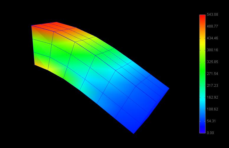
The following model extends FemBeam to render stress, with an added color bar. The loaded model is shown in Figure 6.13.
Chapter 7 DICOM Images
Some models are derived from image data, and it may be useful to show the model and image in the same space. For this purpose, a DICOM image widget has been designed, capable of displaying 3D DICOM volumes as a set of three perpendicular planes. An example widget and its property panel is shown in Figure 7.1.
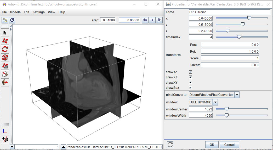
The main classes related to the reading and displaying of DICOM images are:
- DicomElement
-
Describes a single attribute in a DICOM file. - DicomHeader
-
Contains all header attributes (all but the image data) extracted from a DICOM file. - DicomPixelBuffer
-
Contains the decoded image pixels for a single image frame. - DicomSlice
-
Contains both the header and image information for a single 2D DICOM slice. - DicomImage
-
Container for DICOM slices, creating a 3D volume (or 3D + time) - DicomReader
-
Parses DICOM files and folders, appending information to a DicomImage. - DicomViewer
-
Displays the DicomImage in the viewer.
If the purpose is simply to display a DICOM volume in the ArtiSynth viewer, then only the last three classes will be of interest. Readers who simply want to display a DICOM image in their model can skip to Section 7.3.
7.1 The DICOM file format
For a complete description of the DICOM format, see the specification page at http://medical.nema.org/standard.html. A brief description is provided here. Another excellent resource is the blog by Roni Zaharia: http://dicomiseasy.blogspot.ca/.
Each DICOM file contains a number of concatenated attributes (a.k.a. elements), one of which defines the embedded binary image pixel data. The other attributes act as meta-data, which can contain identity information of the subject, equipment settings when the image was acquired, spatial and temporal properties of the acquisition, voxel spacings, etc.... The image data typically represents one or more 2D images, concatenated, representing slices (or ‘frames’) of a 3D volume whose locations are described by the meta-data. This image data can be a set of raw pixel values, or can be encoded using almost any image-encoding scheme (e.g. JPEG, TIFF, PNG). For medical applications, the image data is typically either raw or compressed using a lossless encoding technique. Complete DICOM acquisitions are typically separated into multiple files, each defining one or few frames. The frames can then be assembled into 3D image ‘stacks’ based on the meta-information, and converted into a form appropriate for display.
| VR | Description |
|---|---|
| CS | Code String |
| DS | Decimal String |
| DT | Date Time |
| IS | Integer String |
| OB | Other Byte String |
| OF | Other Float String |
| OW | Other Word String |
| SH | Short String |
| UI | Unique Identifier |
| US | Unsigned Short |
| OX | One of OB, OW, OF |
Each DICOM attribute is composed of:
-
•
a standardized unique integer tag in the format (XXXX,XXXX) that defines the group and element of the attribute
-
•
a value representation (VR) that describes the data type and format of the attribute’s value (see Table 7.1)
-
•
a value length that defines the length in bytes of the attribute’s value to follow
-
•
a value field that contains the attribute’s value
This layout is depicted in Figure 7.2. A list of important attributes are provided in Table 7.2.
| Tag | VR | Value Length | Value Field |
| Attribute name | VR | Tag | |
|---|---|---|---|
| Transfer syntax UID | UI | 0x0002 , | 0x0010 |
| Slice thickness | DS | 0x0018 , | 0x0050 |
| Spacing between slices | DS | 0x0018 , | 0x0088 |
| Study ID | SH | 0x0020 , | 0x0010 |
| Series number | IS | 0x0020 , | 0x0011 |
| Aquisition number | IS | 0x0020 , | 0x0012 |
| Image number | IS | 0x0020 , | 0x0013 |
| Image position patient | DS | 0x0020 , | 0x0032 |
| Image orientation patient | DS | 0x0020 , | 0x0037 |
| Temporal position identifier | IS | 0x0020 , | 0x0100 |
| Number of temporal positions | IS | 0x0020 , | 0x0105 |
| Slice location | DS | 0x0020 , | 0x1041 |
| Samples per pixel | US | 0x0028 , | 0x0002 |
| Photometric interpretation | CS | 0x0028 , | 0x0004 |
| Planar configuration (color) | US | 0x0028 , | 0x0006 |
| Number of frames | IS | 0x0028 , | 0x0008 |
| Rows | US | 0x0028 , | 0x0010 |
| Columns | US | 0x0028 , | 0x0011 |
| Pixel spacing | DS | 0x0028 , | 0x0030 |
| Bits allocated | US | 0x0028 , | 0x0100 |
| Bits stored | US | 0x0028 , | 0x0101 |
| High bit | US | 0x0028 , | 0x0102 |
| Pixel representation | US | 0x0028 , | 0x0103 |
| Pixel data | OX | 0x7FE0 , | 0x0010 |
7.2 The DICOM classes
Each DicomElement represents a single attribute contained in a DICOM file. The DicomHeader contains the collection of DicomElements defined in a file, apart from the pixel data. The image pixels are decoded and stored in a DicomPixelBuffer. Each DicomSlice contains a DicomHeader, as well as the decoded DicomPixelBuffer for a single slice (or ‘frame’). All slices are assembled into a single DicomImage, which can be used to extract 3D voxels and spatial locations from the set of slices. These five classes are described in further detail in the following sections.
7.2.1 DicomElement
The DicomElement class is a simple container for DICOM attribute information. It has three main properties:
-
•
an integer tag
-
•
a value representation (VR)
-
•
a value
These properties can be obtained using the corresponding get function: getTag(), getVR(), getValue(). The tag refers to the concatenated group/element tag. For example, the transfer syntax UID which corresponds to group 0x0002 and element 0x0010 has a numeric tag of 0x00020010. The VR is represented by an enumerated type, DicomElement.VR. The ‘value’ is the raw value extracted from the DICOM file. In most cases, this will be a String. For raw numeric values (i.e. stored in the DICOM file in binary form) such as the unsigned short (US), the ‘value’ property is exactly the numeric value.
For VRs such as the integer string (IS) or decimal string (DS), the string will still need to be parsed in order to extract the appropriate sequence of numeric values. There are static utility functions for handling this within DicomElement. For a ‘best-guess’ of the desired parsed value based on the VR, one can use the method getParsedValue(). Often, however, the desired value is also context-dependent, so the user should know a priori what type of value(s) to expect. Parsing can also be done automatically by querying for values directly through the DicomHeader object.
7.2.2 DicomHeader
When a DICOM file is parsed, all meta-data (attributes apart from the actual pixel data) is assembled into a DicomHeader object. This essentially acts as a map that can be queried for attributes using one of the following methods:
The first method returns the full element as described in the previous section. The remaining methods are used for convenience when the desired value type is known for the given tag. These methods automatically parse or convert the DicomElement’s value to the desired form.
If the tag does not exist in the header, then the getIntValue(...) and getDecimalValue(...) will return the supplied defaultValue. All other methods will return null.
7.2.3 DicomPixelBuffer
The DicomPixelBuffer contains the decoded image information of an image slice. There are three possible pixel types currently supported:
-
•
byte grayscale values (PixelType.BYTE)
-
•
short grayscale values (PixelType.SHORT)
-
•
byte RGB values, with layout RGBRGB...RGB (PixelType.BYTE_RGB)
The pixel buffer stores all pixels in one of these types. The pixels can be queried for directly using getPixel(idx) to get a single pixel, or getBuffer() to get the entire pixel buffer. Alternatively, a DicomPixelInterpolator object can be passed in to convert between pixel types via one of the following methods:
These methods populate an output array or buffer with converted pixel values, which can later be passed to a renderer. For further details on these methods, refer to the Javadoc documentation.
7.2.4 DicomSlice
A single DICOM file contains both header information, and one or more image ‘frames’ (slices). In ArtiSynth, we separate each frame and attach them to the corresponding header information in a DicomSlice. Thus, each slice contains a single DicomHeader and DicomPixelBuffer. These can be obtained using the methods: getHeader() and getPixelBuffer().
For convenience, the DicomSlice also has all the same methods for extracting and converting between pixel types as the DicomPixelBuffer.
7.2.5 DicomImage
An complete DICOM acquisition typically consists of multiple slices forming a 3D image stack, and potentially contains multiple 3D stacks to form a dynamic 3D+time image. The collection of DicomSlices are thus assembled into a DicomImage, which keeps track of the spatial and temporal positions.
The DicomImage is the main object to query for pixels in 3D(+time). To access pixels, it has the following methods:
The inputs {x, y, z} refer to voxel indices, and time refers to the time instance index, starting at zero. The four voxel dimensions of the image can be queried with: getNumCols() getNumRows(), getNumSlices(), and getNumTimes().
The DicomImage also contains spatial transform information for converting between voxel indices and patient-centered spatial locations. The affine transform can be acquired with the method getPixelTransform(). This allows the image to be placed in the appropriate 3D location, to correspond with any derived data such as segmentations. The spatial transformation is automatically extracted from the DICOM header information embedded in the files.
7.3 Loading a DicomImage
DICOM files and folders are read using the DicomReader class. The reader populates a supplied DicomImage with slices, forming the full 3D(+time) image. The basic pattern is as follows:
The first argument in the read(...) command is an existing image in which to append slices. In this case, we pass in null to signal that a new image is to be created.
In some cases, we might wish to exclude certain files, such as meta-data files that happen to be in the DICOM folder. By default, the reader attempts to read all files in a given directory, and will print out an error message for those it fails to detect as being in a valid DICOM format. To limit the files to be considered, we allow the specification of a Java Pattern, which will test each filename against a regular expression. Only files with names that match the pattern will be included. For example, in the following, we limit the reader to files ending with the ``dcm'' extension.
The pattern is applied to the absolute filename, with either windows and mac/linux file separators (both are checked against the regular expression). The method also has an option to recursively search for files in subdirectories. If the full list of files is known, then one can use the method:
which will load all specified files.
7.3.1 Time-dependent images
In most cases, time-dependent images will be properly assembled using the previously mentioned methods in the DicomReader. Each slice should have a temporal position identifier that allows for the separate image stacks to be separated. However, we have found in practice that at times, the temporal position identifier is omitted. Instead, each stack might be stored in a separate DICOM folder. For this reason, additional read methods have been added that allow manual specification of the time index:
If the supplied temporalPosition is non-negative, then the temporal position of all included files will be manually set to that value. If negative, then the method will attempt to read the temporal position from the DICOM header information. If no such information is available, then the reader will guess the temporal position to be one past the last temporal position in the original image stack (or 0 if im == null). For example, if the original image has temporal positions {0, 1, 2}, then all appended slices will have a temporal position of three.
7.3.2 Image formats
The DicomReader attempts to automatically decode any pixel information embedded in the DICOM files. Unfortunately, there are virtually an unlimited number of image formats allowed in DICOM, so there is no way to include native support to decode all of them. By default, the reader can handle raw pixels, and any image format supported by Java’s ImageIO framework, which includes JPEG, PNG, BMP, WBMP, and GIF. Many medical images, however, rely on lossless or near-lossless encoding, such as lossless JPEG, JPEG 2000, or TIFF. For these formats, we provide an interface that interacts with the third-party command-line utilies provided by ImageMagick (http://www.imagemagick.org). To enable this interface, the ImageMagick utilities identify and convert must be available and exist somewhere on the system’s PATH environment variable.
ImageMagick Installation
To enable ImageMagick decoding, required for image formats not natively supported by Java (e.g. JPEG 2000, TIFF), download and install the ImageMagick command-line utilities from: http://www.imagemagick.org/script/binary-releases.php
The install path must also be added to your system’s PATH environment variable so that ArtiSynth can locate the identify and convert utilities.
7.4 The DicomViewer
Once a DicomImage is loaded, it can be displayed in a model by using the DicomViewer component. The viewer has several key properties:
- name
-
the name of the viewer component
- x, y, z
-
the normalized slice positions, in the range [0,1], at which to display image planes
- timeIndex
-
the temporal position (image stack) to display
- transform
-
an affine transformation to apply to the image (on top of the voxel-to-spatial transform extracted from the DICOM file)
- drawYZ
-
draw the YZ plane, corresponding to position x
- drawXZ
-
draw the XZ plane, corresponding to position y
- drawXY
-
draw the XY plane, corresponding to position z
- drawBox
-
draw the 3D image’s bounding box
- pixelConverter
-
the interpolator responsible for converting pixels decoded in the DICOM slices into values appropriate for display. The converter has additional properties:
- window
-
name of a preset window for linear interpolation of intensities
- center
-
center intensity
- width
-
width of window
Each property has a corresponding getXxx(...) and setXxx(...) method that can adjust the settings in code. They can also be modified directly in the ArtiSynth GUI. The last property, the pixelConverter allows for shifting and scaling intensity values for display. By default a set of intensity ‘windows’ are loaded directly from the DICOM file. Each window has a name, and defines a center and width used for linearly scale the intensity range. In addition to the windows extracted from the DICOM, two new windows are added: FULL_DYNAMIC, corresponding to the entire intensity range of the image; and CUSTOM, which allows for custom specification of the window center and width properties.
To add a DicomViewer to the model, create the viewer by supplying a component name and reference to a DicomImage, then add it as a Renderable to the RootModel:
The image will automatically be displayed in the patient-centered coordinates loaded from the DicomImage. In addition to this basic construction, there are convenience constructors to avoid the need for a DicomReader for simple DICOM files:
These constructors generate a new DicomImage internal to the viewer. The image can be retreived from the viewer using the getImage() method.
7.5 DICOM example
Examples of DICOM use can be found in the artisynth.core.demos.dicom package. These demos automatically download sample DICOM data from http://www.osirix-viewer.com/datasets/. The following listing provides one such example, loading an MR image of the wrist. Note that the image data in this example is encoded with the JPEG 2000 format, so ImageMagick is required to decode the pixels (see Section 7.3.2).
Lines 27–33 are responsible for downloading and extracting the sample DICOM zip file. In the end, dicomPath contains a reference to the desired DICOM directory on the local system. On line 36, we create a regular expression pattern that will only match files ending in .dcm. On line 39, we create the viewer, which will automatically parse the desired DICOM files and create a DicomImage internally. We then add the viewer to the model for display purposes. This model is displayed in Figure 7.3.
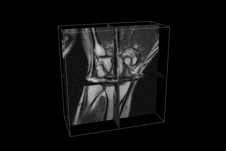
Appendix A Mathematical Review
This appendix reviews some of the mathematical concepts used in this manual.
A.1 Rotation transforms
Rotation matrices are used to describe the orientation of 3D coordinate frames in space, and to transform vectors between these coordinate frames.

Consider two 3D coordinate frames A and B that are rotated with
respect to each other (Figure A.1). The orientation
of B with respect to A can be described by a ![]() rotation
matrix
rotation
matrix ![]() , whose columns are the unit vectors giving the
directions of the rotated axes
, whose columns are the unit vectors giving the
directions of the rotated axes ![]() ,
, ![]() , and
, and ![]() of B with
respect to A.
of B with
respect to A.
![]() is an orthogonal matrix, meaning that
its columns are both perpendicular and mutually
orthogonal, so that
is an orthogonal matrix, meaning that
its columns are both perpendicular and mutually
orthogonal, so that
| (A.1) |
where ![]() is the
is the ![]() identity matrix. The inverse
of
identity matrix. The inverse
of ![]() is hence equal to its transpose:
is hence equal to its transpose:
| (A.2) |
Because ![]() is orthogonal,
is orthogonal, ![]() , and because it
is a rotation,
, and because it
is a rotation, ![]() (the other case, where
(the other case, where ![]() , is not a rotation but a reflection). The 6 orthogonality
constraints associated with a rotation matrix mean that in spite of
having 9 numbers, the matrix only has 3 degrees of freedom.
, is not a rotation but a reflection). The 6 orthogonality
constraints associated with a rotation matrix mean that in spite of
having 9 numbers, the matrix only has 3 degrees of freedom.
Now, assume we have a 3D vector ![]() , and consider its coordinates
with respect to both frames A and B. Where necessary, we use a
preceding superscript to indicate the coordinate frame with respect to
which a quantity is described, so that
, and consider its coordinates
with respect to both frames A and B. Where necessary, we use a
preceding superscript to indicate the coordinate frame with respect to
which a quantity is described, so that ![]() and
and ![]() and
denote
and
denote ![]() with respect to frames A and B, respectively. Given the
definition of
with respect to frames A and B, respectively. Given the
definition of ![]() given above, it is fairly straightforward to
show that
given above, it is fairly straightforward to
show that
| (A.3) |
and, given (A.2), that
| (A.4) |
Hence in addition to describing the orientation of B with respect to A,
![]() is also a transformation matrix that maps vectors in B
to vectors in A.
is also a transformation matrix that maps vectors in B
to vectors in A.
It is straightforward to show that
| (A.5) |

A simple rotation by an angle ![]() about one of the basic
coordinate axes is known as a basic rotation. The three
basic rotations about x, y, and z are:
about one of the basic
coordinate axes is known as a basic rotation. The three
basic rotations about x, y, and z are:
 |
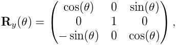 |
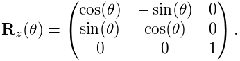 |
Next, we consider transform composition. Suppose we have three
coordinate frames, A, B, and C, whose orientation are related to each other by
![]() ,
, ![]() , and
, and ![]() (Figure
A.6). If we know
(Figure
A.6). If we know ![]() and
and ![]() ,
then we can determine
,
then we can determine ![]() from
from
| (A.6) |
This can be understood in terms of vector transforms. ![]() transforms a vector from C to B, which is equivalent to first
transforming from C to A,
transforms a vector from C to B, which is equivalent to first
transforming from C to A,
| (A.7) |
and then transforming from A to B:
| (A.8) |
Note also from (A.5) that ![]() can be
expressed as
can be
expressed as
| (A.9) |
In addition to specifying rotation matrix components explicitly, there are numerous other ways to describe a rotation. Three of the most common are:
- Roll-pitch-yaw angles
-
There are 6 variations of roll-pitch-yaw angles. The one used in ArtiSynth corresponds to older robotics texts (e.g., Paul, Spong) and consists of a roll rotation
 about the z axis, followed by a pitch
rotation
about the z axis, followed by a pitch
rotation  about the new y axis, followed by a yaw rotation
  about the new x axis. The net rotation can be expressed by the
following product of basic rotations:
about the new x axis. The net rotation can be expressed by the
following product of basic rotations: 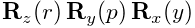 .
. - Axis-angle
-
An axis angle rotation parameterizes a rotation as a rotation by an angle
about a specific axis  . Any rotation
can be represented in such a way as a consequence of Euler’s rotation
theorem.
. Any rotation
can be represented in such a way as a consequence of Euler’s rotation
theorem. - Euler angles
-
There are 6 variations of Euler angles. The one used in ArtiSynth consists of a rotation
about the z axis, followed by a rotation
about the new y axis, followed by a rotation  about the
new z axis. The net rotation can be expressed by the following product
of basic rotations:
about the
new z axis. The net rotation can be expressed by the following product
of basic rotations: 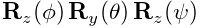 .
.
A.2 Rigid transforms
Rigid transforms are used to specify both the transformation of points and vectors between coordinate frames, as well as the relative position and orientation between coordinate frames.

Consider two 3D coordinate frames in space, A and B (Figure
A.3). The translational position of B with respect to A
can be described by a vector ![]() from the origin of A to the
origin of B (described with respect to frame A). Meanwhile, the
orientation of B with respect to A can be described by the
from the origin of A to the
origin of B (described with respect to frame A). Meanwhile, the
orientation of B with respect to A can be described by the ![]() rotation matrix
rotation matrix ![]() (Section A.1). The
combined position and orientation of B with respect to A is known as
the pose of B with respect to A.
(Section A.1). The
combined position and orientation of B with respect to A is known as
the pose of B with respect to A.

Now, assume we have a 3D point ![]() , and consider its coordinates with
respect to both frames A and B (Figure A.4). Given the
pose descriptions given above, it is fairly straightforward to show
that
, and consider its coordinates with
respect to both frames A and B (Figure A.4). Given the
pose descriptions given above, it is fairly straightforward to show
that
| (A.10) |
and, given (A.2), that
| (A.11) |
If we extend our points into a 4D homogeneous coordinate space
with the fourth coordinate ![]() equal to 1, i.e.,
equal to 1, i.e.,
 |
(A.12) |
then (A.10) and (A.11) can be simplified to
where
 |
(A.13) |
and
 |
(A.14) |
![]() is the
is the ![]() rigid transform matrix that
transforms points from B to A and also describes the pose of
B with respect to A (Figure A.5).
rigid transform matrix that
transforms points from B to A and also describes the pose of
B with respect to A (Figure A.5).

It is straightforward to show that ![]() and
and ![]() describe the orientation and position of
describe the orientation and position of ![]() with respect to
with respect to
![]() , and so therefore
, and so therefore
| (A.15) |
Note that if we are transforming a vector ![]() instead of a point
between B and A, then we are only concerned about relative orientation
and the vector transforms (A.3) and
(A.4) should be used instead.
However, we can express these using
instead of a point
between B and A, then we are only concerned about relative orientation
and the vector transforms (A.3) and
(A.4) should be used instead.
However, we can express these using ![]() if
we embed vectors in a homogeneous coordinate space
with the fourth coordinate
if
we embed vectors in a homogeneous coordinate space
with the fourth coordinate ![]() equal to 0, i.e.,
equal to 0, i.e.,
|
(A.16) |
so that

A.3 Affine transforms
An affine transform is a generalization of a rigid transform, in
which the rotational component ![]() is replaced by a general
is replaced by a general ![]() matrix
matrix ![]() . This means that an affine transform implements a
generalized basis transformation combined with an offset of the origin
(Figure A.7). As with
. This means that an affine transform implements a
generalized basis transformation combined with an offset of the origin
(Figure A.7). As with ![]() for rigid transforms, the
columns of
for rigid transforms, the
columns of ![]() still describe the transformed basis vectors
still describe the transformed basis vectors ![]() ,
,
![]() , and
, and ![]() , but these are generally no longer orthonormal.
, but these are generally no longer orthonormal.

Expressed in terms of homogeneous coordinates,
the affine transform ![]() takes the form
takes the form
 |
(A.18) |
with
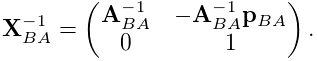 |
(A.19) |
As with rigid transforms, when an affine transform is applied to a
vector instead of a point, only the matrix ![]() is applied and the
translation component
is applied and the
translation component ![]() is ignored.
is ignored.
Affine transforms are typically used to effect transformations that
require stretching and shearing of a coordinate frame. By the polar
decomposition theorem, ![]() can be factored into a regular
rotation
can be factored into a regular
rotation ![]() plus a symmetric shearing/scaling matrix
plus a symmetric shearing/scaling matrix ![]() :
:
| (A.20) |
Affine transforms can also be used to perform reflections, in which
![]() is orthogonal (so that
is orthogonal (so that ![]() ) but with
) but with ![]() .
.
A.4 Rotational velocity

Given two 3D coordinate frames A and B, the rotational, or angular, velocity of B with respect to A is given by a 3D vector
![]() (Figure A.8).
(Figure A.8). ![]() is related to the derivative of
is related to the derivative of ![]() by
by
| (A.21) |
where ![]() and
and ![]() indicate
indicate ![]() with
respect to frames
with
respect to frames ![]() and
and ![]() and
and ![]() denotes the
denotes the ![]() cross product matrix
cross product matrix
![[\boldsymbol{\omega}]\equiv\left(\begin{matrix}0&-\omega_{z}&\omega_{y}\\
\omega_{z}&0&-\omega_{x}\\
-\omega_{y}&\omega_{x}&0\\
\end{matrix}\right).](mi/mi16.png) |
(A.22) |
If we consider instead the velocity of ![]() with respect to
with respect to ![]() , it is
straightforward to show that
, it is
straightforward to show that
| (A.23) |
A.5 Spatial velocities and forces
Given two 3D coordinate frames A and B, the spatial velocity,
or twist,
![]() of B with respect to A is given by the 6D
composition of the translational velocity
of B with respect to A is given by the 6D
composition of the translational velocity ![]() of the
origin of B with respect to A and the angular velocity
of the
origin of B with respect to A and the angular velocity ![]() :
:
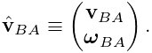 |
(A.24) |
Similarly, the spatial force, or wrench, ![]() acting
on a frame B is given by the 6D composition of the translational force
acting
on a frame B is given by the 6D composition of the translational force
![]() acting on the frame’s origin and the moment
acting on the frame’s origin and the moment ![]() , or torque,
acting through the frame’s origin:
, or torque,
acting through the frame’s origin:
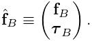 |
(A.25) |
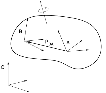
If we have two frames ![]() and
and ![]() rigidly connected within a rigid
body (Figure A.9), and we know the spatial velocity
rigidly connected within a rigid
body (Figure A.9), and we know the spatial velocity
![]() of
of ![]() with respect to some third frame
with respect to some third frame ![]() , we may wish
to know the spatial velocity
, we may wish
to know the spatial velocity ![]() of
of ![]() with respect to
with respect to ![]() .
The angular velocity components are the same, but the translational
velocity components are coupled by the angular velocity and the offset
.
The angular velocity components are the same, but the translational
velocity components are coupled by the angular velocity and the offset
![]() between
between ![]() and
and ![]() , so that
, so that
![]() is hence related to
is hence related to ![]() via
via
![\left(\begin{matrix}{\bf v}_{AC}\\
\boldsymbol{\omega}_{AC}\end{matrix}\right)=\left(\begin{matrix}{\bf I}&[{\bf p%
}_{BA}]\\
0&{\bf I}\end{matrix}\right)\,\left(\begin{matrix}{\bf v}_{BC}\\
\boldsymbol{\omega}_{BC}\end{matrix}\right).](mi/mi37.png) |
where ![]() is defined by
(A.22).
is defined by
(A.22).
The above equation assumes that all quantities are expressed
with respect to the same coordinate frame.
If we instead consider ![]() and
and ![]() to be represented
in frames
to be represented
in frames ![]() and
and ![]() , respectively, then
we can show that
, respectively, then
we can show that
| (A.26) |
where
![{\bf X}_{BA}\equiv\left(\begin{matrix}{\bf R}_{BA}&[{\bf p}_{BA}]{\bf R}_{BA}%
\\
0&{\bf R}_{BA}\end{matrix}\right).](mi/mi78.png) |
(A.27) |
The transform ![]() is easily formed from the components of the
rigid transform
is easily formed from the components of the
rigid transform ![]() relating
relating ![]() to
to ![]() .
.
The spatial forces ![]() and
and ![]() acting on frames
acting on frames ![]() and
and
![]() within a rigid body are related in a similar way, only with
spatial forces, it is the moment that is coupled through the moment
arm created by
within a rigid body are related in a similar way, only with
spatial forces, it is the moment that is coupled through the moment
arm created by ![]() , so that
, so that
If we again assume that ![]() and
and ![]() are expressed in frames
are expressed in frames ![]() and
and ![]() , we can show that
, we can show that
| (A.28) |
where
![{\bf X}^{*}_{BA}\equiv\left(\begin{matrix}{\bf R}_{BA}&0\\
~{}[{\bf p}_{BA}]{\bf R}_{BA}&{\bf R}_{BA}\end{matrix}\right).](mi/mi76.png) |
(A.29) |
A.6 Spatial inertia
Assume we have a rigid body with mass ![]() and a coordinate frame
located at the body’s center of mass. If
and a coordinate frame
located at the body’s center of mass. If ![]() and
and ![]() give the
translational and rotational velocity of the coordinate frame, then
the body’s linear and angular momentum
give the
translational and rotational velocity of the coordinate frame, then
the body’s linear and angular momentum ![]() and
and ![]() are given by
are given by
| (A.30) |
where ![]() is the
is the ![]() rotational inertia with respect
to the center of mass. These relationships can be combined into a
single equation
rotational inertia with respect
to the center of mass. These relationships can be combined into a
single equation
| (A.31) |
where ![]() and
and ![]() are the spatial momentum and
spatial inertia:
are the spatial momentum and
spatial inertia:
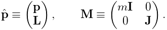 |
(A.32) |
The spatial momentum satisfies Newton’s second law, so that
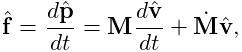 |
(A.33) |
which can be used to find the acceleration of a body in response to a spatial force.
When the body coordinate frame is not located at the center of mass, then the spatial inertia assumes the more complicated form
![\left(\begin{matrix}m{\bf I}&-m[{\bf c}]\\
m[{\bf c}]&{\bf J}-m[{\bf c}][{\bf c}]\end{matrix}\right),](mi/mi35.png) |
(A.34) |
where ![]() is the center of mass and
is the center of mass and ![]() is defined by
(A.22).
is defined by
(A.22).
Like the rotational inertia, the spatial inertia is always symmetric
positive definite if ![]() .
.
Bibliography
- [1] (2002) A time-stepping method for stiff multibody dynamics with contact and friction. International Journal for Numerical Methods in Engineering 55 (7), pp. 753–784. Cited by: 4.6.3.
- [2] (2005) Three-dimensional representation of complex muscle architectures and geometries. Annals of biomedical engineering 33 (5), pp. 661–673. Cited by: 6.8.3.
- [3] (2000) Nonlinear continuum mechanics for finite element analysis. Cambridge University Press. Cited by: 6.1.
- [4] (2007) Ghosts and machines: regularized variational methods for interactive simulations of multibodies with dry frictional contacts. Ph.D. Thesis, Datavetenskap, UmeÂ, Computer Science Dept., Umea University, Sweden. Cited by: 4.6.3.
- [5] (2012) ArtiSynth: a fast interactive biomechanical modeling toolkit combining multibody and finite element simulation. In Soft tissue biomechanical modeling for computer assisted surgery, pp. 355–394. Cited by: 1.2.
- [6] (2008-Feb.) Efficient deformable body simulation using stiffness-warped nonlinear finite elements. In Symposium on Interactive 3D Graphics and Games (i3D), pp. . Note: poster Cited by: 6.1.3.
- [7] (2006) A linearly implicit trapezoidal method for integrating stiff multibody dynamics with contact, joints, and friction. International Journal for Numerical Methods in Engineering 66 (7), pp. 1079–1124. Cited by: 4.6.3.
![[LOGO]](data:image/png;base64,iVBORw0KGgoAAAANSUhEUgAAAAsAAAAOCAYAAAD5YeaVAAAAAXNSR0IArs4c6QAAAAZiS0dEAP8A/wD/oL2nkwAAAAlwSFlzAAALEwAACxMBAJqcGAAAAAd0SU1FB9wKExQZLWTEaOUAAAAddEVYdENvbW1lbnQAQ3JlYXRlZCB3aXRoIFRoZSBHSU1Q72QlbgAAAdpJREFUKM9tkL+L2nAARz9fPZNCKFapUn8kyI0e4iRHSR1Kb8ng0lJw6FYHFwv2LwhOpcWxTjeUunYqOmqd6hEoRDhtDWdA8ApRYsSUCDHNt5ul13vz4w0vWCgUnnEc975arX6ORqN3VqtVZbfbTQC4uEHANM3jSqXymFI6yWazP2KxWAXAL9zCUa1Wy2tXVxheKA9YNoR8Pt+aTqe4FVVVvz05O6MBhqUIBGk8Hn8HAOVy+T+XLJfLS4ZhTiRJgqIoVBRFIoric47jPnmeB1mW/9rr9ZpSSn3Lsmir1fJZlqWlUonKsvwWwD8ymc/nXwVBeLjf7xEKhdBut9Hr9WgmkyGEkJwsy5eHG5vN5g0AKIoCAEgkEkin0wQAfN9/cXPdheu6P33fBwB4ngcAcByHJpPJl+fn54mD3Gg0NrquXxeLRQAAwzAYj8cwTZPwPH9/sVg8PXweDAauqqr2cDjEer1GJBLBZDJBs9mE4zjwfZ85lAGg2+06hmGgXq+j3+/DsixYlgVN03a9Xu8jgCNCyIegIAgx13Vfd7vdu+FweG8YRkjXdWy329+dTgeSJD3ieZ7RNO0VAXAPwDEAO5VKndi2fWrb9jWl9Esul6PZbDY9Go1OZ7PZ9z/lyuD3OozU2wAAAABJRU5ErkJggg==)