7.6 Visualizing fields
It is often useful to be able to visualize the contents of a field, particularly for testing and validation purposes. ArtiSynth field components export various properties that allow their values to be visualized in the viewer.
As described in Section 7.6.3, the grid field components, ScalarGridField and VectorGridField, are not visible by default, and so must be made visible to enable visualization.
7.6.1 Scalar fields
Scalar fields are visualized by means of a color map that associates scalar values with colors, with the actually visualization typically taking the form of either a discrete set of colored points, or a colored surface embedded within the field. The color map and its associated visualization is controlled by the following properties:
- colorMap
-
An instance of the ColorMap interface that controls how field values are mapped onto colors. Various types of maps exist, including GreyscaleColorMap, HueColorMap, RainbowColorMap, and JetColorMap, each containing subproperties controlling how its colors are generated.
- renderRange
-
Composite property of the type ScalarRange that controls the range of field values used for color map rendering. Subproperties include interval, which gives the value range itself, and updating, which specifies how this interval is determined from the field: FIXED (interval can be set manually), AUTO_EXPAND (interval is expanded to accommodate all field values), and AUTO_FIT (interval is tightly fit to the field values). Note that for AUTO_EXPAND and AUTO_FIT, the interval is determined by the range of field values, and not the values that actually appear in the visualization. The latter can differ from the former when the surface does not cover the whole field, or lies outside the field, resulting in extrapolated values that fall outside the field’s range. Setting updating to FIXED and manually setting the interval can be useful in such cases.
- visualization
-
An enumerated type that specifies the actual type of rendering used to visualize the field (e.g., points, surface, or other). While its definition is specific to the field type (ScalarFemField.Visualization for FEM fields, ScalarMeshField.Visualization for mesh fields; ScalarGridField.Visualization for grid fields), overall it will have one of five values (POINT, SURFACE, ELEMENT, FACE, or OFF) described further below.
- volumeElemsVisible
-
A boolean property, exported by ScalarElementField and ScalarSubElemField, which if false causes volumetric element values to be ignored in the visualization. The default value is true.
- shellElemsVisible
-
A boolean property, exported by ScalarElementField and ScalarSubElemField, which if false causes shell element values to be ignored in the visualization. The default value is true.
- renderProps
-
Basic rendering properties of the field component that are used to control some aspects of the rendering (Section 4.3), as described below.
The above properties can be accessed either interactively in the GUI, or in code, using the field’s methods getColorMap(), setColorMap(map), getRenderRange(), setRenderRange(range), getVisualization(), and setVisualization(type).
While the enumerated type associated with the visualization property is specific to the field type, all values together will be one of the following:
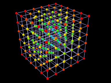
- POINT
-
Field is visualized using colored points placed at the features used to define the field (e.g., nodes, element centers, or integration points for FEM fields; vertices and face centers for mesh fields; vertices for grid fields). How the points are displayed is controlled using the pointStyle subproperty of the grid’s renderProps, with their size controlled either by pointRadius or pointSize (if the pointStyle is POINT).
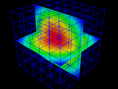
- SURFACE
-
Field is visualized using a colored surface, specified by one or more polygonal meshes associated with the field, where the values at mesh vertices are either determined directly, or interpolated from, the field. This type of visualization is available for ScalarNodalField, ScalarSubElemField, ScalarVertexField and ScalarGridField. For ScalarVertexField, the mesh is the mesh associated with the field itself. Otherwise, the meshes are supplied by external mesh components that are attached to the field as render meshes, as described in Section 7.6.4. For ScalarNodalField and ScalarSubElemField, these mesh components must be either FemMeshComps (Section 6.3) or FemCutPlanes (Section 6.12.7) associated with the FEM model, and may include its surface mesh; while for ScalarGridField, the mesh components are fixed mesh bodies (Section 3.3.1).
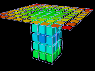
- ELEMENT
-
Used only by ScalarElementField, allows the field to be visualized by element shaped widgets that are colored according to each element’s field value and the color map. The size of the widget, relative to the true element size, is controlled by the property elementWidgetSize, which is a scalar in the range
![[0,1]](mi/mi2248.png) .
. - FACE
-
Used only by ScalarFaceField, allows the field to be visualized by rendering the associated field mesh, with each face colored according to its field value and the color map.
- OFF
-
No visualization (the default value).
7.6.2 Vector fields
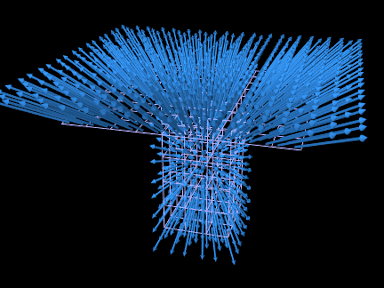
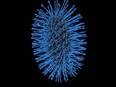
Vector fields can be visualized, when possible, by drawing three dimensional line segments, with a length proportional to the field value, originating at the features used to define the field (nodes, element centers, or integration points for FEM fields; vertices and face centers for mesh fields; vertices for grid fields). This can done for any field whose vector type is an instance of Vector (which includes Vector2d, Vector3d, and VectorNd) by mapping the vector values onto a 3-vector. This means ignoring element values for vectors whose size is greater than 3, and setting higher element values to 0 for vectors whose size is less than 3.
Vector field rendering is controlled by the following properties:
- renderScale
-
A double which scales the vector field value to determine the length of the drawn line segment. The default value is 0, implying that no vectors are drawn.
- renderProps
-
Basic rendering properties of the field component, as described in Section 4.3. How the lines are displayed is controlled by the line subproperties, with the color specified by lineColor, the style by lineStyle (LINE, CYLINDER, SOLID_ARROW, SPINDLE), and the size by either lineRadius or lineWidth (if the lineStyle is LINE).
7.6.3 Grid fields
As mentioned above, the grid field components, ScalarGridField and VectorGridField, are not visible by default, and so must be made visible to enable visualization:
By default, grid field components also render their grid edges, using the edge subproperties of renderProps (drawEdges, edgeWidth, and edgeColor). If edgeColor is not set (i.e., is set to null), the lineColor subproperty is used instead. Grid components also have a renderGrid property which can be set to false to disable rendering of the grid.
For VectorGridField, when rendering the grid and visualizing the vectors, one can make them different colors by using the edgeColor subproperty of renderProps to set the grid color:
7.6.4 Render meshes
The scalar fields ScalarNodalField, ScalarSubElemField, and ScalarGridField all make use of render meshes when being visualized using SURFACE visualization. These are a collection of one or more components, each providing a polygonal mesh that defines a surface for rendering a color map of the field, based on values at the mesh vertices that are themselves determined from the field. For ScalarNodalField and ScalarSubElemField), the mesh components must be either FemMeshComps contained within the FEM’s meshes list (Section 6.3) or FemCutPlanes contained within the FEM’s cutPlanes list (Section 6.12.7), while for ScalarGridField, they are FixedMeshBodys (Section 3.3.1) that are usually contained within the MechModel.
Adding render meshes to a field must be done in code. For ScalarNodalField and ScalarSubElemField, the set of rendering meshes is controlled by the following methods:
| void addRenderMeshComp (FemMesh mcomp) |
Add the render mesh component mcomp. |
| boolean removeRenderMeshComp (FemMesh mcomp) |
Remove the render mesh component mcomp. |
| FemMesh getRenderMeshComp (idx) |
Return the idx-th render mesh component. |
| int numRenderMeshComps() |
Return the number of render mesh components. |
| void clearRenderMeshComps() |
Clear all the render mesh components. |
Equivalent methods exist for ScalarGridField, using FixedMeshBody instead of FemMesh.
The following should be noted with respect to render meshes:
-
•
A render mesh can be created for the sole purpose of visualizing a field. A rectangle often does well for this purpose.
-
•
Rendering of the visualization is done by the field component, not the render mesh component(s), and so it is usually necessary to make the latter invisible to avoid rendering conflicts.
-
•
Render meshes should have a large enough number of vertices and triangles to support the resolution required to visualize the field properly.
-
•
One can often use the GUI transformer tools to interactively adjust a render mesh’s pose (see “Transformer tools” in the ArtiSynth User Interface Guide), allowing the user to move a render surface throughout the field. For FixedMeshBody and FemCutPlane, the tools change the component’s pose, while for FemMeshComp, they change the location of its embedding within the FEM.
Transformer tools have no effect on FEM meshes which are auto-generated, such as the default surface mesh.
As a simple example, the following code fragment creates a square render mesh for a ScalarGridField:
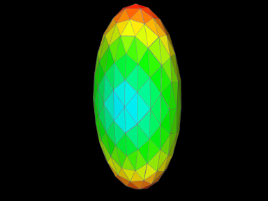
7.6.5 Example: Visualizing a scalar nodal field
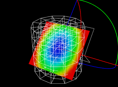
A simple application that uses a FemCutPlane to visualize a ScalarNodalField is defined in
artisynth.demos.tutorial.ScalarFieldVisualization
The build() method for this is shown below:
After first creating a MechModel (lines 2-3), a cylindrical
hexahedral FEM model is created to contain the field, with its top
nodes fixed to allow it to deform under gravity (lines 13-17). A ScalarNodalField is then defined for this FEM, where the value at
each node is set to ![]() , with
, with ![]() being the radial distance from the
node to the FEM’s central axis (lines 21-27).
being the radial distance from the
node to the FEM’s central axis (lines 21-27).
To visualize the field, a FemCutPlane is created with its pose
set to align it with the ![]() -
-![]() plane and then added to the FEM model
(lines 31-33). The field’s visualization is then set to SURFACE
and the cut plane is added to it as a render mesh (lines 36-37). At
lines 40-44, a control panel is created to allow interactive
adjustment of the field’s visualization, renderRange, and
colorMap properties. Finally, render properties are set: the FEM
line color (used to render element edges) is set to blue-gray (line
48); the cut plane’s surface rendering is set to None to avoid
interfering with the field rendering, and axis rendering is enabled to
make the field visible and selectable even if it doesn’t intersect the
FEM (lines 51-53); and, for POINT visualization, the field is
set to render points as spheres with a radius of
plane and then added to the FEM model
(lines 31-33). The field’s visualization is then set to SURFACE
and the cut plane is added to it as a render mesh (lines 36-37). At
lines 40-44, a control panel is created to allow interactive
adjustment of the field’s visualization, renderRange, and
colorMap properties. Finally, render properties are set: the FEM
line color (used to render element edges) is set to blue-gray (line
48); the cut plane’s surface rendering is set to None to avoid
interfering with the field rendering, and axis rendering is enabled to
make the field visible and selectable even if it doesn’t intersect the
FEM (lines 51-53); and, for POINT visualization, the field is
set to render points as spheres with a radius of ![]() (line 55).
(line 55).
To run this example in ArtiSynth, select All demos > tutorial > ScalarFieldVisualization from the Models menu. Users can employ the control panel to adjust the visualization, the render range, and the color map. When SURFACE visualization is selected, the field will be rendered onto the FEM/plane intersection defined by the cut plane. Simulating the model will cause the FEM to deform, deforming this intersection with it. Clicking on the intersection surface or the cut plane axes will cause the cut plane to be selected. Its pose can then be adjusted using the GUI transformer tools (see “Model Manipulation” in the ArtiSynth User Interface Guide), as shown in Figure 7.3.
When the updating property of the render range is set to AUTO_FIT, the range will be automatically set to the range of values in the field, and not the values evaluated over the render surface. The latter may exceed the former due to extrapolation when the surface extends outside of the FEM, in which case the visualization will appear to saturate. While this is not generally a concern because FEM field values are unreliable outside of the FEM, one can override this effect by setting the updating property to FIXED and setting the range interval manually.
7.6.6 Examples: Visualizing other fields
|
Numerous examples exist for creating and visualizing other field types:
  artisynth.demos.fem.ScalarNodalFieldDemo
  artisynth.demos.fem.ScalarElementFieldDemo
  artisynth.demos.fem.ScalarSubElemFieldDemo
  artisynth.demos.fem.VertexNodalFieldDemo
  artisynth.demos.fem.VertexElementFieldDemo
  artisynth.demos.fem.VertexSubElemFieldDemo

  artisynth.demos.mech.ScalarVertexFieldDemo
  artisynth.demos.mech.ScalarFaceFieldDemo
  artisynth.demos.mech.ScalarGridFieldDemo
  artisynth.demos.mech.VertexVertexFieldDemo
  artisynth.demos.mech.VertexFaceFieldDemo
  artisynth.demos.mech.VertexGridFieldDemo
|
|
![[LOGO]](data:image/png;base64,iVBORw0KGgoAAAANSUhEUgAAAAsAAAAOCAYAAAD5YeaVAAAAAXNSR0IArs4c6QAAAAZiS0dEAP8A/wD/oL2nkwAAAAlwSFlzAAALEwAACxMBAJqcGAAAAAd0SU1FB9wKExQZLWTEaOUAAAAddEVYdENvbW1lbnQAQ3JlYXRlZCB3aXRoIFRoZSBHSU1Q72QlbgAAAdpJREFUKM9tkL+L2nAARz9fPZNCKFapUn8kyI0e4iRHSR1Kb8ng0lJw6FYHFwv2LwhOpcWxTjeUunYqOmqd6hEoRDhtDWdA8ApRYsSUCDHNt5ul13vz4w0vWCgUnnEc975arX6ORqN3VqtVZbfbTQC4uEHANM3jSqXymFI6yWazP2KxWAXAL9zCUa1Wy2tXVxheKA9YNoR8Pt+aTqe4FVVVvz05O6MBhqUIBGk8Hn8HAOVy+T+XLJfLS4ZhTiRJgqIoVBRFIoric47jPnmeB1mW/9rr9ZpSSn3Lsmir1fJZlqWlUonKsvwWwD8ymc/nXwVBeLjf7xEKhdBut9Hr9WgmkyGEkJwsy5eHG5vN5g0AKIoCAEgkEkin0wQAfN9/cXPdheu6P33fBwB4ngcAcByHJpPJl+fn54mD3Gg0NrquXxeLRQAAwzAYj8cwTZPwPH9/sVg8PXweDAauqqr2cDjEer1GJBLBZDJBs9mE4zjwfZ85lAGg2+06hmGgXq+j3+/DsixYlgVN03a9Xu8jgCNCyIegIAgx13Vfd7vdu+FweG8YRkjXdWy329+dTgeSJD3ieZ7RNO0VAXAPwDEAO5VKndi2fWrb9jWl9Esul6PZbDY9Go1OZ7PZ9z/lyuD3OozU2wAAAABJRU5ErkJggg==)