7.5 Binding material properties
A principal purpose of field components is to enable certain FEM material properties to vary spatially over the FEM geometry. Many material properties can be bound to a field, so that when they are queried internally by the solver at the integration points for each FEM element, the field value at that integration point is used instead of the regular property value. Likewise, some properties of contact force behaviors, such as the YoungsModulus and thickness properties of LinearElasticContact (Section 8.7.3) can be bound to a field that varies over the contact mesh geometry.
To bind a property to a field, it is necessary that
-
1.
The type of the field matches the value of the property;
-
2.
The property is itself bindable.
If the property has a double value, then it can be bound to any ScalarFieldComponent. Otherwise, if the property has a value T, where T is an instance of maspack.matrix.VectorObject, then it can be bound to a vector field.
Bindable properties export two methods with the signature
where XXX is the property name and F is an appropriate field type.
As long as a property XXX is bound to a field, its regular value will still appear (and can be set) through widgets in control or property panels, or via its getXXX() and setXXX() accessors. However, the regular value won’t be used internally by the FEM simulation.
For example, consider the YoungsModulus property, which is present in several FEM materials, including LinearMaterial and NeoHookeanMaterial. This has a double value, and is bindable, and so can be bound to a ScalarFieldComponent as follows:
It is important to perform field bindings on materials before they are set in an FEM model (or one of its subcomponents, such as MuscleBundles). That’s because the setMaterial() method copies the input material, and so any settings made on it afterwards won’t be seen by the FEM:
   // works: field will be seen by the copied version of ’mat’
   mat.setYoungsModulusField (field);
   fem.setMaterial (mat);

   // does NOT work: field not seen by the copied version of ’mat’
   fem.setMaterial (mat);
   mat.setYoungsModulusField (field);
To unbind YoungsModulus, one can call
Usually, FEM fields are used to bind properties in FEM materials while mesh fields are used for contact properties, but other fields can be used, particularly grid fields. To understand this a bit better, we discuss briefly some of the internals of how binding works. When evaluating stresses, FEM materials have access to a FemFieldPoint object that provides information about the integration point, including its element, nodal weights, and integration point index. This can be used to rapidly evaluate values within nodal, element and sub-element FEM fields. Likewise, when evaluating contact forces, contact materials like LinearElasticContact have access to a MeshFieldPoint object that describes the contact point position as a weighted sum of mesh vertex positions, which can then be used to rapidly evaluate values within vertex or face mesh fields. However, all fields, regardless of type, implement methods for determining values at both FemFieldPoints and MeshFieldPoints:
If necessary, these methods simply fall back on the getValue(Point3d) method, which is defined for all fields and works relatively fast for grid fields.
There are some additional details to consider when binding FEM material properties:
-
1.
When binding to a grid field, one has the choice of whether to use the grid to represent values with respect to the FEM’s rest position or spatial position. This can be controlled by setting the useFemRestPositions property of the grid field, the default value for which is true.
-
2.
When binding the bulkModulus property of an incompressible material, it is best to use a nodal field if the FEM model is using nodal-based soft incompressibility (i.e., the model’s softIncompMethod property is set to either NODAL or AUTO; Section 6.7.3). That’s because soft nodal incompressibility requires evaluating the bulk modulus property at nodes instead of integration points, which is much easier to do with a nodal-based field.
7.5.1 Example: FEM with variable stiffness
A simple model demonstrating a stiffness that varies over an FEM mesh is defined in
artisynth.demos.tutorial.VariableStiffness
It consists of a simple thin hexahedral beam with a linear material
for which the Young’s modulus ![]() is made to vary nonlinearly along the
x axis of the rest position according to the formula
is made to vary nonlinearly along the
x axis of the rest position according to the formula
| (7.0) |
The model’s build method is given below:
Lines 6-10 create the hex FEM model and shift it so that the left side
is aligned with the origin, while lines 12-17 fix the leftmost
nodes. Lines 21-27 create a scalar nodal field for the Young’s modulus,
with lines 23-24 computing ![]() according to (7.0).
The field is then bound to a linear material which is then set in the
model (lines 30-32).
according to (7.0).
The field is then bound to a linear material which is then set in the
model (lines 30-32).
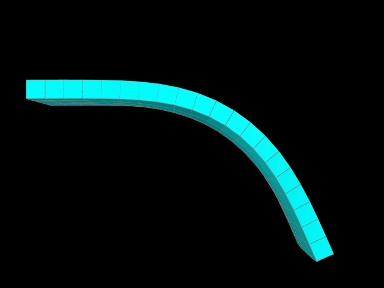
The example can be run in ArtiSynth by selecting All demos > tutorial > VariableStiffness from the Models menu. When run, the beam will bend under gravity, but mostly on the right side, due to the much higher stiffness on the left (Figure 7.1).
7.5.2 Example: specifying FEM muscle directions
 |
 |
Another example involves using a Vector3d field to specify the muscle activation directions over an FEM model and is defined in
artisynth.demos.tutorial.RadialMuscle
When muscles are added using MuscleBundles ( Section 6.9), the muscle directions are stored and handled internally by the muscle bundle itself. However, it is possible to add a MuscleMaterial directly to the elements of an FEM model, using a MaterialBundle (Section 6.8), in which case the directions need to be set explicitly using a field.
The model’s build method is given below:
Lines 5-19 create a thin cylindrical FEM model, centered on the
origin, with radius ![]() and height
and height ![]() , consisting of hexes with
wedges at the center, with two layers of elements along the
, consisting of hexes with
wedges at the center, with two layers of elements along the ![]() axis
(which is parallel to the cylinder axis). Its base material is set to
a neo-hookean material. To keep the model from falling under gravity,
all nodes whose distance to the
axis
(which is parallel to the cylinder axis). Its base material is set to
a neo-hookean material. To keep the model from falling under gravity,
all nodes whose distance to the ![]() axis is less than
axis is less than ![]() are fixed.
are fixed.
Next, a Vector3d field is created to specify the directions, on a
per-element basis, for the muscle material which will be added subsequently
(lines 21-32). While we could create an instance of VectorElementField<Vector3d>, we use
Vector3dElementField, since this
is available and provides additional functionality (such as the
ability to render the directions). Directions are set to lie outward
in a radial direction perpendicular to the ![]() axis, and since the
model is centered on the origin, they can be computed easily by first
computing the element centroids, removing the
axis, and since the
model is centered on the origin, they can be computed easily by first
computing the element centroids, removing the ![]() component, and then
normalizing. In order to give the muscle action an upward bias, we
only set directions for elements in the upper layer. Direction values
for elements in the lower layer will then automatically have a default
value of 0, which will cause the muscle material to not apply any
stress.
component, and then
normalizing. In order to give the muscle action an upward bias, we
only set directions for elements in the upper layer. Direction values
for elements in the lower layer will then automatically have a default
value of 0, which will cause the muscle material to not apply any
stress.
We next add to the model a muscle material whose directions will be determined by the field. To hold the material, we first create and add a MaterialBundle which is set to act on all elements (line 35-36). Then we set this bundle’s material to SimpleForceMuscle, which adds a stress along the muscle direction that equals the excitation value times the value of its maxStress property, and bind the material’s restDir property to the direction field (lines 37-39).
Finally, we create and add a control panel to allow interactive control over the muscle material’s excitation property (lines 42-44), and set some rendering properties for the FEM model.
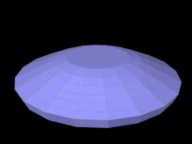
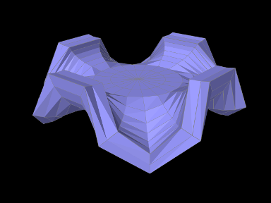
The example can be run in ArtiSynth by selecting All demos > tutorial > RadialMuscle from the Models menu. When it is first run, it falls around the edges under gravity (Figure 7.2, top). Applying an excitation causes a radial contraction which pulls the edges upward and, if high enough, causes them to buckle (Figure 7.2, bottom).
![[LOGO]](data:image/png;base64,iVBORw0KGgoAAAANSUhEUgAAAAsAAAAOCAYAAAD5YeaVAAAAAXNSR0IArs4c6QAAAAZiS0dEAP8A/wD/oL2nkwAAAAlwSFlzAAALEwAACxMBAJqcGAAAAAd0SU1FB9wKExQZLWTEaOUAAAAddEVYdENvbW1lbnQAQ3JlYXRlZCB3aXRoIFRoZSBHSU1Q72QlbgAAAdpJREFUKM9tkL+L2nAARz9fPZNCKFapUn8kyI0e4iRHSR1Kb8ng0lJw6FYHFwv2LwhOpcWxTjeUunYqOmqd6hEoRDhtDWdA8ApRYsSUCDHNt5ul13vz4w0vWCgUnnEc975arX6ORqN3VqtVZbfbTQC4uEHANM3jSqXymFI6yWazP2KxWAXAL9zCUa1Wy2tXVxheKA9YNoR8Pt+aTqe4FVVVvz05O6MBhqUIBGk8Hn8HAOVy+T+XLJfLS4ZhTiRJgqIoVBRFIoric47jPnmeB1mW/9rr9ZpSSn3Lsmir1fJZlqWlUonKsvwWwD8ymc/nXwVBeLjf7xEKhdBut9Hr9WgmkyGEkJwsy5eHG5vN5g0AKIoCAEgkEkin0wQAfN9/cXPdheu6P33fBwB4ngcAcByHJpPJl+fn54mD3Gg0NrquXxeLRQAAwzAYj8cwTZPwPH9/sVg8PXweDAauqqr2cDjEer1GJBLBZDJBs9mE4zjwfZ85lAGg2+06hmGgXq+j3+/DsixYlgVN03a9Xu8jgCNCyIegIAgx13Vfd7vdu+FweG8YRkjXdWy329+dTgeSJD3ieZ7RNO0VAXAPwDEAO5VKndi2fWrb9jWl9Esul6PZbDY9Go1OZ7PZ9z/lyuD3OozU2wAAAABJRU5ErkJggg==)