6 Finite Element Models 6 Finite Element Models 6.2 FEM model creation

6.1 Overview

The finite element method (FEM) is a numerical technique used for solving a system of partial differential equations (PDEs) over some domain. The general approach is to divide the domain into a set of building blocks, referred to as elements. These partition the space, and form local domains over which the system of equations can be locally approximated. The corners of these elements, the nodes, become control points in a discretized system. The solution is then assumed to be smoothly interpolated across the elements based on values determined at the nodes. Using this discretization, the differential system is converted into an algebraic one, which is often linearized and solved iteratively.

In ArtiSynth, the PDEs considered are the governing equations of continuum mechanics: the conservation of mass, momentum, and energy. To complete the system, a constitutive equation is required that describes the stress-strain response of the material. This constitutive equation is what distinguishes between material types. The domain is the three-dimensional space that the model occupies. This must be divided into small elements which accurately represent the geometry. Within each element, the PDEs are sampled at a set of points, referred to as integration points, and terms are numerically integrated to form an algebraic system to solve.

The purpose of the rest of this chapter is to describe the construction and use of finite elements models within ArtiSynth. It does not further discuss the mathematical framework or theory. For an in-depth coverage of the nonlinear finite element method, as applied to continuum mechanics, the reader is referred to the textbook by Bonet and Wood [5].

6.1.1 FemModel3d

The basic type of finite element model is implemented in the class FemModel3d. This class controls some properties that are used by the model as a whole. The key ones that affect simulation dynamics are:

Property	Description
density	The density of the model
material	An object that describes the material’s constitutive law (i.e. its stress-strain relationship).
particleDamping	Proportional damping associated with the particle-like motion of the FEM nodes.
stiffnessDamping	Proportional damping associated with the system’s stiffness term.

These properties can be set and retrieved using the methods

void setDensity (double density)	Sets the density.
double getDensity()	Gets the density.
@VERTSPACE[0.5em]
void setMaterial (FemMaterial mat)	Sets the FEM’s material.
FemMaterial getMaterial()	Gets the FEM’s material.
@VERTSPACE[0.5em]
void setParticleDamping (double d)	Sets the particle (mass) damping.
double getParticleDamping()	Gets the particle (mass) damping.
@VERTSPACE[0.5em]
void setStiffnessDamping (double d)	Sets the stiffness damping.
double getStiffnessDamping()	Gets the stiffness damping.

Keep in mind that ArtiSynth is essentially “unitless” (Section 4.2), so it is the responsibility of the developer to ensure that all properties are specified in a compatible way.

The density of the model is used to compute the mass distribution throughout the volume. Note that we use a diagonally lumped mass matrix (DLMM) formulation, so the mass is assumed to be concentrated at the location of the discretized FEM nodes. To allow for a spatially-varying density, densities can be explicitly set for individual elements, or masses can be explicitly set for individual nodes.

The FEM’s material property is a delegate object used to compute stress and stiffness within individual elements. It handles the constitutive component of the model, as described in more detail in Section 6.1.3. In addition to the main material defined for the model, it is also possible set a material on a per-element basis, and to define additional materials which augment the behavior of the main materials (Section 6.8).

The two damping parameters are related to Rayleigh damping, which is used to dissipate energy within finite element models. There are two proportional damping terms: one related to the system’s mass, and one related to stiffness. The resulting damping force applied is

$\displaystyle{\bf f}_{d}$

$\displaystyle=-(d_{M}{\bf M}+d_{K}{\bf K}){\bf v},$

(6.0)

where $d_{M}$ is the value of particleDamping, $d_{K}$ is the value of stiffnessDamping, ${\bf M}$ is the FEM model’s lumped mass matrix, ${\bf K}$ is the FEM’s stiffness matrix, and ${\bf v}$ is the concatenated vector of FEM node velocities. Since the lumped mass matrix is diagonal, the mass-related component of damping can be applied separately to each FEM node. Thus, the mass component reduces to the same system as Equation (3.3), which is why it is referred to as “particle damping”.

6.1.2 Component Structure

Each FemModel3d contains several lists of subcomponents:

nodes: The particle-like dynamic components of the model. These lie at the corners of the elements and carry all the mass (due to DLMM formulation).
elements: The volumetric model elements. These define the 3D sub-units over which the system is numerically integrated.
shellElements: The shell elements. These define additional 2D sub-units over which the system is numerically integrated.
meshes: The geometry in the model. This includes the surface mesh, and any other embedded geometries.
materials: Optional additional materials which can be added to the model to augment the behavior of the model’s material property. This is described in more detail in Section 6.8.
fields: Optional field components which can be used to interpolate application-defined quantities over the FEM model’s domain. Fields are described in detail in Chapter 7.

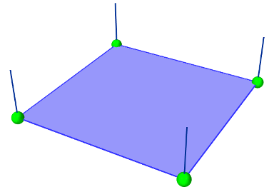
The nodes, elements and meshes components are illustrated in Figure 6.2.


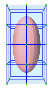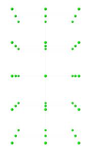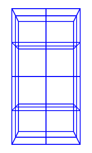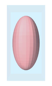(a) FEM model	(b) Nodes	(c) Elements	(d) Geometry

Figure 6.2: Subcomponents of FemModel3d.

6.1.2.1 Nodes

The set of nodes belong to a finite element model can be obtained by the method

PointList<FemNode3d> getNodes()

Returns the list of FEM nodes.

Nodes are implemented in the class FemNode3d, which is a subclass of Particle (Section 3.1). They are the main dynamic components of the finite element model. The key properties affecting simulation dynamics are:

Property	Description
restPosition	The initial position of the node.
position	The current position of the node.
velocity	The current velocity of the node.
mass	The mass of the node.
dynamic	Whether the node is considered dynamic or parametric (e.g. boundary condition).

Each of these properties has corresponding getXxx() and setXxx(...) functions to access and modify them.

The restPosition property defines the node’s position in the FEM model’s “natural” or “undeformed” state. Rest positions are used to compute an initial configuration for the model, from which strains are determined. A node’s rest position can be updated in code using the method: FemNode3d.setRestPosition(Point3d).

If any node’s rest positions are changed, the current values for stress and stiffness will become invalid. They can be manually updated using the method FemModel3d.updateStressAndStiffness() for the parent model. Otherwise, stress and stiffness will be automatically updated at the beginning of the next time step.

The properties position and velocity give the node’s current 3D state. These are common to all point-like particles, as is the mass property. Here, however, mass represents the lumped mass of the immediately surrounding material. Its value is initialized by equally dividing mass contributions from each adjacent element, given their densities. For a finer control of spatially-varying density, node masses can be set manually after FEM creation.

The FEM node’s dynamic property specifies whether or not the node is considered when computing the dynamics of the system. If not, it is treated as being parametrically controlled. This has implications when setting boundary conditions (Section 6.1.4).

6.1.2.2 Elements

Elements are the 3D volumetric spatial building blocks of the domain. Within each element, the displacement (or strain) field is interpolated from displacements at nodes:

$\displaystyle{\bf u}({\bf x})$

$\displaystyle=\sum_{i=1}^{N}\phi_{i}({\bf x}){\bf u}_{i},$

(6.1)

where ${\bf u}_{i}$ is the displacement of the th node that is adjacent to the element, and $\phi_{i}(\cdot)$ is referred to as the shape function (or basis function) associated with that node. Elements are classified by their shape, number of nodes, and shape function order (Table 6.1). ArtiSynth supports the following element types:


TetElement,	PyramidElement,	WedgeElement,	HexElement,
QuadtetElement	QuadpyramidElement	QuadwedgeElement	QuadhexElement

Table 6.1: Supported element types

Element Type	# Nodes	Order	# Integration Points
TetElement	4	linear	1
PyramidElement	5	linear	5
WedgeElement	6	linear	6
HexElement	8	linear	8
QuadtetElement	10	quadratic	4
QuadpyramidElement	13	quadratic	5
QuadwedgeElement	15	quadratic	9
QuadhexElement	20	quadratic	14

The base class for all of these is FemElement3d. A numerical integration is performed within each element to create the (tangent) stiffness matrix. This integration is performed by evaluating the stress and stiffness at a set of integration points within each element, and applying numerical quadrature. The list of elements in a model can be obtained with the method

RenderableComponentList<FemElement3d> getElements()

Returns the list of volumetric elements.

All objects of type FemElement3d have the following properties:

Property	Description
density	Density of the element
material	An object that describes the constitutive law within the element (i.e. its stress-strain relationship).

If left unspecified, the element’s density is inherited from the containing FemModel3d object. When set, the mass of the element is computed and divided amongst all its nodes, updating the lumped mass matrix.

Each element’s material property is also inherited by default from the containing FemModel3d. Specifying a material here allows for spatially-varying material properties across the model. Materials will be discussed further in Section 6.1.3.

6.1.2.3 Shell elements

Shell elements are additional 2D spatial building blocks which can be added to a model. They are typically used to model structures which are too thin to be easily represented by 3D volumetric elements, or to provide additional internal stiffness within a set of volumetric elements.

ArtiSynth presently supports the following shell element types, with the number of nodes, shape function order, and integration point count described in Table 6.2:


ShellTriElement	ShellQuadElement

Table 6.2: Supported shell element types

Element Type	# Nodes	Order	# Integration Points
ShellTriElement	3	linear	9 (3 if membrane)
ShellQuadElement	4	linear	8 (4 if membrane)

The base class for all shell elements is ShellElement3d, which contains the same density and material properties as FemElement3d, as well as the additional property defaultThickness, whose use will be described below.

The list of shell elements in a model can be obtained with the method

RenderableComponentList<ShellElement3d> getShellElements()

Returns the list of shell elements.

Both the volumetric elements (FemElement3d) and the shell elements (ShellElement3d) derive from the base class FemElement3dBase. To obtain all the elements in an FEM model, both shell and volumetric, one may use the method

ArrayList<FemElement3dBase> getAllElements()

Returns a list of all elements.

Each shell element can actually be instantiated in two forms:

•

As a regular shell element, which has a bending stiffness;
•

As a membrane element, which does not have bending stiffness.

Regular shell elements are implemented using the same extensible director formulation used by FEBio [11], and more specifically the front/back node formulation [12]. Each node associated with a (regular) shell element is assigned a director, which is a 3D vector providing a normal direction and virtual thickness at that node (Figure 6.3). This virtual thickness allows us to continue to use 3D materials to provide the constitutive laws that determine the shell’s stress/strain response, including its bending behavior. It also allows us to continue to use the element’s density to determine its mass.

Figure 6.3: ShellQuadElement with the directors (dark blue lines) visible at the nodes.

Director information is automatically assigned to a FemNode3d whenever one or more regular shell elements is connected to it. This information includes both the current value of the director, its rest value, and its velocity, with the difference between the first two determining the element’s bending strain. These quantities can be queried using the methods

⬇

Vector3d getDirector (); // return the current director value

void getDirector (Vector3d dir);

Vector3d getRestDirector (); // return the rest director value

void getRestDirector (Vector3d dir);

Vector3d getDirectorVel (); // return the director velocity

boolean hasDirector(); // does this node have a director?

For nodes which are not connected to regular shell elements, and therefore do not have director information assigned, these methods all return a zero-valued vector.

If not otherwise specified, the current and rest director values are computed automatically from the surrounding (regular) shell elements, with their value ${\bf d}$ being computed from

${\bf d}=\sum t_{i}\,{\bf n}_{i}$

where $t_{i}$ is the value of the defaultThickness property and ${\bf n}_{i}$ is the surface normal of the -th surrounding regular shell element. However, if necessary, it is also possible to explicitly assign these values, using the methods

⬇

setDirector (Vector3d dir); // set the current director

setRestDirector (Vector3d dir); // set the rest director

ArtiSynth FEM nodes can currently support only one director, which is shared by all regular shell elements associated with that node. This effectively means that all such elements must belong to the same “surface”, and that two intersecting surfaces cannot share the same nodes.

As indicated above, shell elements can also be instantiated as membrane elements, which do not exhibit bending stiffness and therefore do not require director information. The regular/membrane distinction is specified in the element’s constructor. For example, ShellTriElement and ShellQuadElement each have constructors with the signatures:

⬇

ShellTriElement (FemNode3d n0, FemNode3d n1, FemNode3d n2,

double thickness, boolean membrane);

ShellQuadElement (FemNode3d n0, FemNode3d n1, FemNode3d n2, FemNode3d n3,

double thickness, boolean membrane);

The thickness argument specifies the defaultThickness property, while membrane determines whether or not the element is a membrane element.

While membrane elements do not require explicit director information stored at the nodes, they do make use of an inferred director that is parallel to the element’s surface normal, and has a constant length equal to the element’s defaultThickness property. This gives the element a virtual volume, which (as with regular elements) is used to determine 3D strains and to compute the element’s mass from it’s density.

6.1.2.4 Meshes

The geometry associated with a finite element model consists of a collection of meshes (e.g. PolygonalMesh, PolylineMesh, PointMesh) that move along with the model in a way that maintains the shape function interpolation equation (6.1) at each vertex location. These geometries can be used for visualizations, or for physical interactions like collisions. However, they have no physical properties themselves. FEM geometries will be discussed in more detail in Section 6.3. The list of meshes can be obtained with the method

⬇

MeshComponentList<FemMeshComp> getMeshComps();

6.1.3 Materials

The stress-strain relationship within each element is defined by a “material” delegate object, implemented by a subclass of FemMaterial. This material object is responsible for implementing the functions

⬇

void computeStressAndTangent (...)

which computes the stress tensor and (optionally) the tangent stiffness matrix at each integration point, based on the current local deformation at that point.

The default material type is LinearMaterial, where stress is related to strain through:

	$\displaystyle\sigma({\bf x})=D\,\epsilon({\bf x}),$		(6.2)
	$\displaystyle\text{where }\quad D=\begin{bmatrix}\lambda+2\mu&\lambda&\lambda&% 0&0&0\\ \lambda&\lambda+2\mu&\lambda&0&0&0\\ \lambda&\lambda&\lambda+2\mu&0&0&0\\ 0&0&0&\mu&0&0\\ 0&0&0&0&\mu&0\\ 0&0&0&0&0&\mu\end{bmatrix},\quad\lambda=\dfrac{E\nu}{(1+\nu)(1-2\nu)},\quad\mu% =\dfrac{E}{2(1+\nu)},$

$\sigma$ is the standard $6\times 1$ stress vector, $\epsilon$ is the strain vector, is the Young’s Modulus, and $\nu$ is Poisson’s ratio. This linear material uses a corotational formulation, so rotations are removed per element before computing the strain [16]. To enable or disable this corotational formulation, use LinearMaterial.setCorotated(boolean).

All material models, including linear and nonlinear, are available in the package artisynth.core.materials. A list of common materials is provided in Table 6.3. Those that are subclasses of IncompressibleMaterial allow for incompressibility.

Table 6.3: Commonly used FEM materials

Material	Parameters
LinearMaterial		Young’s modulus
	$\nu$	Poisson’s ratio
	corotated	corotational formulation
StVenantKirchoffMaterial		Young’s modulus
	$\nu$	Poisson’s ratio
NeoHookeanMaterial		Young’s modulus
	$\nu$	Poisson’s ratio
IncompNeoHookeanMaterial		shear modulus
	$\kappa$	bulk modulus
MooneyRivlinMaterial	$C_{10},C_{01},C_{20},C_{02}$	distortional parameters
	$\kappa$	bulk modulus
OgdenMaterial	$\mu_{1},\ldots,\mu_{6}$	material parameters
	$\alpha_{1},\ldots,\alpha_{6}$
	$\kappa$	bulk modulus

6.1.4 Boundary conditions

Boundary conditions can be implemented in one of several ways:

1.

Explicitly setting FEM node positions/velocities
2.

Attaching FEM nodes to other dynamic components
3.

Enabling collisions

To enforce an explicit (Dirichlet) boundary condition for a set of nodes, their dynamic property must be set to false. This notifies ArtiSynth that the state of these nodes (both position and velocity) will be controlled parametrically. By disabling dynamics, a fixed boundary condition is applied. For a moving boundary, positions and velocities of the boundary nodes must be explicitly set every timestep. This can be accomplished with either a Controller (see Section 5.3) or an InputProbe (see Section 5.4). Note that both the position and velocity of the nodes should be explicitly set for consistency.

Another type of supported boundary condition is to attach FEM nodes to other components, including particles, springs, rigid bodies, and locations within other FEM elements. Here, the node is still considered dynamic, but its motion is coupled to that of the attached component through a constraint mechanism. Attachments will be discussed further in Section 6.4.

Finally, the boundary of an FEM can be constrained by enabling collisions with other components. This will be covered in Chapter 8.

6 Finite Element Models Bibliography 6.2 FEM model creation

Generated on Tue Mar 26 13:12:56 2024 by LaTeXML [LOGO]