6.10 Material types
ArtiSynth FEM models support a variety of material types, including
linear, hyperelastic, and activated muscle materials, described in the
sections below. These can be used to supply the primary material for
either an entire FEM model or for specific elements (using the setMaterial() methods for either). They can also be used to supply
auxiliary materials, whose behavior is superimposed on the underlying
material, via either material bundles
(Section 6.8) or,
for FemMuscleModels, muscle bundles
(Section 6.9). Many of the properties for a given
material can be bound to a scalar or vector field
(Section 7.2) to allow their values to vary across an
FEM model. In the descriptions below, properties for which this is
true will have a ![]() indicated under the “Field” entry in the
material’s property table.
indicated under the “Field” entry in the
material’s property table.
All materials are defined in the package artisynth.core.materials.
6.10.1 Linear
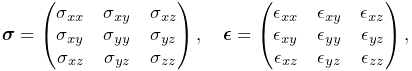
Linear materials determine Cauchy stress ![]() as a linear mapping
from the small deformation Cauchy strain
as a linear mapping
from the small deformation Cauchy strain ![]() ,
,
| (6.7) |
where ![]() is the elasticity tensor.
Both the stress and
strain are symmetric
is the elasticity tensor.
Both the stress and
strain are symmetric ![]() matrices,
matrices,
 |
(6.8) |
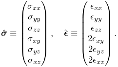
and can be expressed as 6-vectors using Voigt notation:
 |
(6.9) |
This allows the constitutive mapping to be expressed in matrix form as
| (6.10) |
where ![]() is the
is the ![]() elasticity matrix.
elasticity matrix.
Different Voigt notation mappings appear in the literature with regard to off-diagonal matrix entries. We use the one employed by FEBio [13]. Another common mapping is
Traditionally, Cauchy strain is computed from the symmetric part of
the deformation gradient ![]() using the formula
using the formula
| (6.11) |
where ![]() is the
is the ![]() identity matrix. However, ArtiSynth
materials support corotation, in which rotations are first
removed from
identity matrix. However, ArtiSynth
materials support corotation, in which rotations are first
removed from ![]() using a polar decomposition
using a polar decomposition
| (6.12) |
where ![]() is a (right-handed) rotation matrix and
is a (right-handed) rotation matrix and ![]() is a symmetric
matrix.
is a symmetric
matrix. ![]() is then used to compute the Cauchy strain:
is then used to compute the Cauchy strain:
| (6.13) |
Corotation is the default behavior for linear materials in ArtiSynth and allows models to handle large scale rotational deformations [18, 16].
For linear materials, the stress/strain response is computed at a single integration point in the center of each element. This is done
to improve computational efficiency, as it allows the precomputation
of stiffness matrices that map nodal displacements onto nodal forces
for each element. This precomputed matrix can then be adjusted during
each simulation step to account for the rotation ![]() computed at each
element’s integration
point [18, 16].
computed at each
element’s integration
point [18, 16].
Specific linear material types are listed in the subsections below. All are subclasses of LinearMaterialBase, and in addition to their individual properties, all export a corotation property (default value true) that controls whether corotation is applied.
6.10.1.1 LinearMaterial
LinearMaterial is a standard isotropic linear material, which is also the default material for FEM models. Its elasticity matrix is given by
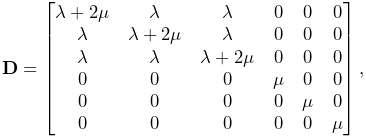 |
(6.14) |
where the Lamé parameters ![]() and
and ![]() are
derived from Young’s modulus
are
derived from Young’s modulus ![]() and Poisson’s ratio
and Poisson’s ratio ![]() via
via
| (6.15) |
The material behavior is controlled by the following properties:
| Property | Description | Default | Field | |
|---|---|---|---|---|
| YoungsModulus | Young’s modulus | 500000 | ✓ | |
| PoissonsRatio | Poisson’s ratio | 0.33 | ||
| corotated | applies corotation if true | true |
LinearMaterials can be created with the following constructors:
| LinearMaterial() |
Create with default properties. |
| LinearMaterial (double E, double nu) |
Create with specified |
| LinearMaterial (double E, double nu, boolean corotated) |
Create with specified |
6.10.1.2 TransverseLinearMaterial
TransverseLinearMaterial
is a transversely isotropic linear material whose behavior is
symmetric about a prescribed polar axis. If the polar axis is
parallel to the ![]() axis, then the elasticity matrix is specified most
easily in terms of its inverse, or compliance matrix, according
to
axis, then the elasticity matrix is specified most
easily in terms of its inverse, or compliance matrix, according
to
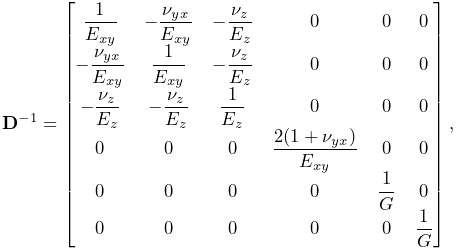 |
where ![]() and
and ![]() are Young’s moduli transverse
and parallel to the axis, respectively,
are Young’s moduli transverse
and parallel to the axis, respectively, ![]() and
and ![]() are
Poisson’s ratios transverse and parallel to the axis, and
are
Poisson’s ratios transverse and parallel to the axis, and ![]() is the
shear modulus.
is the
shear modulus.
The material behavior is controlled by the following properties:
| Property | Description | Default | Field | |
|---|---|---|---|---|
| youngsModulus | Young’s moduli transverse and parallel to the axis | ✓ | ||
| poissonsRatio | Poisson’s ratios transverse and parallel to the axis | |||
| shearModulus | shear modulus | 187970 | ✓ | |
| direction | direction of the polar axis | ✓ | ||
| corotated | applies corotation if true | true |
The youngsModulus and poissonsRatio properties are both described by Vector2d objects, while direction is described by a Vector3d. The direction property (as well as youngsModulus and shearModulus) can be bound to a field to allow its value to vary over an FEM model (Section 7.2).
TransverseLinearMaterials can be created with the following constructors:
| TransverseLinearMaterial() |
Create with default properties. |
| TransverseLinearMaterial (Vector2d E, double G, Vector2d nu, boolean corotated) |
Create with specified |
6.10.1.3 AnisotropicLinearMaterial
AnisotropicLinearMaterial
is a general anisotropic linear material whose behavior is specified
by an arbitrary (symmetric) elasticity matrix ![]() .
The material behavior is controlled by the following properties:
.
The material behavior is controlled by the following properties:
| Property | Description | Default | Field | |
|---|---|---|---|---|
| stiffnessTensor | symmetric |
|||
| corotated | applies corotation if true | true |
The default value for stiffnessTensor is an isotropic elasticity
matrix corresponding to ![]() and
and ![]() .
.
AnisotropicLinearMaterials can be created with the following constructors:
| AnisotropicLinearMaterial() |
Create with default properties. |
| AnisotropicLinearMaterial (Matrix6dBase D) |
Create with specified elasticity |
| AnisotropicLinearMaterial (Matrix6dBase D, boolean corotated) |
Create with specified |
6.10.2 Hyperelastic materials
A hyperelastic material is defined by a strain energy density
function ![]() that is in general a function of the deformation gradient
that is in general a function of the deformation gradient
![]() , and more specifically a quantity derived from
, and more specifically a quantity derived from ![]() that is
rotationally invariant, such as the right Cauchy Green
tensor
that is
rotationally invariant, such as the right Cauchy Green
tensor ![]() , the left Cauchy Green
tensor
, the left Cauchy Green
tensor ![]() , or Green strain
, or Green strain
| (6.15) |
![]() is often described with respect to the first or second invariants
of these quantities, denoted by
is often described with respect to the first or second invariants
of these quantities, denoted by ![]() and
and ![]() and defined with
respect to a given matrix
and defined with
respect to a given matrix ![]() by
by
| (6.16) |
Alternatively, ![]() is sometimes defined with respect to the three
principal stretches of the deformation,
is sometimes defined with respect to the three
principal stretches of the deformation, ![]() , which are the eigenvalues of the symmetric component
, which are the eigenvalues of the symmetric component ![]() of the
polar decomposition of
of the
polar decomposition of ![]() in (6.12).
in (6.12).
If ![]() is expressed with respect to
is expressed with respect to ![]() , then the second
Piola-Kirchhoff stress
, then the second
Piola-Kirchhoff stress ![]() is given by
is given by
| (6.17) |
from which the Cauchy stress can be obtained via
| (6.18) |
Many of the hyperelastic materials described below are incompressible, in the sense that ![]() is partitioned into a deviatoric component that is volume invariant and a dilational
component that depends solely on volume changes.
Volume change is
characterized by
is partitioned into a deviatoric component that is volume invariant and a dilational
component that depends solely on volume changes.
Volume change is
characterized by ![]() , with the change in volume given by
, with the change in volume given by ![]() and
and ![]() indicating no volume change. Deviatoric
changes are characterized by
indicating no volume change. Deviatoric
changes are characterized by ![]() , with
, with
| (6.19) |
and so the partitioned strain energy density function assumes the form
| (6.20) |
where the ![]() term is the deviatoric contribution and
term is the deviatoric contribution and
![]() is the volumetric potential that enforces incompressibility.
is the volumetric potential that enforces incompressibility.
![]() may also be expressed with respect to the right deviatoric
Cauchy Green tensor
may also be expressed with respect to the right deviatoric
Cauchy Green tensor ![]() or the left deviatoric Cauchy Green
tensor
or the left deviatoric Cauchy Green
tensor ![]() , respectively defined by
, respectively defined by
| (6.21) |
ArtiSynth supplies different forms of ![]() , as specified by a
material’s bulkPotential property and detailed in
Section 6.7.3. All of the available potentials depend
on a bulkModulus property
, as specified by a
material’s bulkPotential property and detailed in
Section 6.7.3. All of the available potentials depend
on a bulkModulus property ![]() , and so
, and so ![]() is often
expressed as
is often
expressed as ![]() . A larger bulk modulus will make the
material more incompressible, with effective incompressibility
typically achieved by setting
. A larger bulk modulus will make the
material more incompressible, with effective incompressibility
typically achieved by setting ![]() to a value that exceeds the
other elastic moduli in the material by a factor of 100 or more.
All incompressible materials are subclasses of
IncompressibleMaterialBase.
to a value that exceeds the
other elastic moduli in the material by a factor of 100 or more.
All incompressible materials are subclasses of
IncompressibleMaterialBase.
6.10.2.1 St Venant-Kirchoff material
StVenantKirchoffMaterial
is a compressible isotropic material that extends isotropic linear
elasticity to large deformations.
The strain energy density is most easily expressed as a function
of the Green strain ![]() :
:
| (6.22) |
where the Lamé parameters ![]() and
and ![]() are
derived from Young’s modulus
are
derived from Young’s modulus ![]() and Poisson’s ratio
and Poisson’s ratio ![]() according to (6.15).
From this definition it follows that the second Piola-Kirchhoff stress
tensor is given by
according to (6.15).
From this definition it follows that the second Piola-Kirchhoff stress
tensor is given by
| (6.23) |
The material behavior is controlled by the following properties:
| Property | Description | Default | Field | |
|---|---|---|---|---|
| YoungsModulus | Young’s modulus | 500000 | ✓ | |
| PoissonsRatio | Poisson’s ratio | 0.33 |
StVenantKirchoffMaterials can be created with the following constructors:
| StVenantKirchoffMaterial() |
Create with default properties. |
| StVenantKirchoffMaterial (double E, double nu) |
Create with specified elasticity |
6.10.2.2 Neo-Hookean material
NeoHookeanMaterial
is a compressible isotropic material with a strain energy density
expressed as a function of the first invariant ![]() of the right
Cauchy-Green tensor
of the right
Cauchy-Green tensor ![]() and
and ![]() :
:
| (6.23) |
where the Lamé parameters ![]() and
and ![]() are derived from
Young’s modulus
are derived from
Young’s modulus ![]() and Poisson’s ratio
and Poisson’s ratio ![]() via
(6.15). The Cauchy stress can be expressed in terms of
the left Cauchy-Green tensor
via
(6.15). The Cauchy stress can be expressed in terms of
the left Cauchy-Green tensor ![]() as
as
| (6.24) |
The material behavior is controlled by the following properties:
| Property | Description | Default | Field | |
|---|---|---|---|---|
| YoungsModulus | Young’s modulus | 500000 | ✓ | |
| PoissonsRatio | Poisson’s ratio | 0.33 |
NeoHookeanMaterials can be created with the following constructors:
| NeoHookeanMaterial() |
Create with default properties. |
| NeoHookeanMaterial (double E, double nu) |
Create with specified elasticity |
6.10.2.3 Incompressible neo-Hookean material
IncompNeoHookeanMaterial
is an incompressible version of the neo-Hookean material,
with a strain energy density expressed in terms of the
first invariant ![]() of the deviatoric
right Cauchy-Green tensor
of the deviatoric
right Cauchy-Green tensor ![]() , plus a potential
function
, plus a potential
function ![]() to enforce incompressibility:
to enforce incompressibility:
| (6.24) |
The material behavior is controlled by the following properties:
| Property | Description | Default | Field | |
|---|---|---|---|---|
| shearModulus | shear modulus | 150000 | ✓ | |
| bulkModulus | bulk modulus for incompressibility | 100000 | ✓ | |
| bulkPotential | incompressibility potential function |
QUADRATIC |
IncompNeoHookeanMaterials can be created with the following constructors:
| IncompNeoHookeanMaterial() |
Create with default properties. |
| IncompNeoHookeanMaterial (double G, double kappa) |
Create with specified elasticity |
6.10.2.4 Mooney-Rivlin material
MooneyRivlinMaterial
is an incompressible isotropic material with a strain energy density
expressed as a polynomial of the first and second invariants ![]() and
and ![]() of the right deviatoric Cauchy-Green
tensor
of the right deviatoric Cauchy-Green
tensor ![]() . ArtiSynth supplies a five parameter version of this
model, with a strain energy density given by
. ArtiSynth supplies a five parameter version of this
model, with a strain energy density given by
| (6.24) |
A two-parameter version (![]() ,
, ![]() ) is often found in the
literature, consisting of only the first two terms:
) is often found in the
literature, consisting of only the first two terms:
| (6.25) |
The material behavior is controlled by the following properties:
| Property | Description | Default | Field | |
|---|---|---|---|---|
| C10 | first coefficient | 150000 | ✓ | |
| C01 | second coefficient | 0 | ✓ | |
| C11 | third coefficient | 0 | ✓ | |
| C20 | fourth coefficient | 0 | ✓ | |
| C02 | fifth coefficient | 0 | ✓ | |
| bulkModulus | bulk modulus for incompressibility | 100000 | ✓ | |
| bulkPotential | incompressibility potential function |
QUADRATIC |
MooneyRivlinMaterials can be created with the following constructors:
| MooneyRivlinMaterial() |
Create with default properties. |
| MooneyRivlinMaterial (double C10, double C01, double C11, double C20, double C02, double kappa) |
Create with specified coefficients. |
6.10.2.5 Ogden material
OgdenMaterial
is an incompressible material with a strain energy density
expressed as a function of the deviatoric principal stretches ![]() :
:
 |
(6.25) |
ArtiSynth allows a maximum of six terms, corresponding to ![]() , and
the material behavior is controlled by the following properties:
, and
the material behavior is controlled by the following properties:
| Property | Description | Default | Field | |
|---|---|---|---|---|
| Mu1 | first multiplier | 300000 | ✓ | |
| Mu2 | second multiplier | 0 | ✓ | |
| ... | ... | ... | 0 | ✓ |
| Mu6 | final multiplier | 0 | ✓ | |
| Alpha1 | first multiplier | 2 | ✓ | |
| Alpha2 | second multiplier | 2 | ✓ | |
| ... | ... | ... | 2 | ✓ |
| Alpha6 | final multiplier | 2 | ✓ | |
| bulkModulus | bulk modulus for incompressibility | 100000 | ✓ | |
| bulkPotential | incompressibility potential function |
QUADRATIC |
OgdenMaterials can be created with the following constructors:
| OgdenMaterial() |
Create with default properties. |
| OgdenMaterial (double[] mu, double[] alpha, double kappa) |
Create with specified |
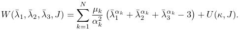
6.10.2.6 Fung orthotropic material
FungOrthotropicMaterial
is an incompressible orthotropic material defined with respect to an
![]() -
-![]() -
-![]() coordinate system expressed by a
coordinate system expressed by a ![]() rotation
matrix
rotation
matrix ![]() . The strain energy density is expressed as a function of
the deviatoric Green strain
. The strain energy density is expressed as a function of
the deviatoric Green strain
| (6.25) |
and the three unit direction vectors ![]() representing the columns of
representing the columns of ![]() . Letting
. Letting ![]() and defining
and defining
| (6.26) |
the energy density is given by
 |
(6.27) |
where ![]() is a material coefficient and
is a material coefficient and ![]() and
and ![]() are
the orthotropic Lamé parameters.
are
the orthotropic Lamé parameters.
At present, the coordinate frame ![]() is not defined in the material,
but can be specified on a per-element basis using the element method
setFrame(Matrix3dBase). For example:
is not defined in the material,
but can be specified on a per-element basis using the element method
setFrame(Matrix3dBase). For example:
One should be careful to ensure that the argument to setFrame() is in fact an orthogonal rotation matrix as this will not be otherwise enforced.
The material behavior is controlled by the following properties:
| Property | Description | Default | Field | |
|---|---|---|---|---|
| mu1 | second Lamé parameter along |
1000 | ✓ | |
| mu2 | second Lamé parameter along |
1000 | ✓ | |
| mu3 | second Lamé parameter along |
1000 | ✓ | |
| lam11 | first Lamé parameter along |
2000 | ✓ | |
| lam22 | first Lamé parameter along |
2000 | ✓ | |
| lam33 | first Lamé parameter along |
2000 | ✓ | |
| lam12 | first Lamé parameter for |
2000 | ✓ | |
| lam23 | first Lamé parameter for |
2000 | ✓ | |
| lam31 | first Lamé parameter for |
2000 | ✓ | |
| C | C coefficient | 1500 | ✓ | |
| bulkModulus | bulk modulus for incompressibility | 100000 | ✓ | |
| bulkPotential | incompressibility potential function |
QUADRATIC |
FungOrthotropicMaterials can be created with the following constructors:
| FungOrthotropicMaterial() |
Create with default properties. |
| FungOrthotropicMaterial (double mu1, double mu2, double mu3, double lam11, double lam22, double lam33, double lam12, double lam23, double lam31, double C, double kappa) |
Create with specified properties. |
6.10.2.7 Yeoh material
YeohMaterial is an incompressible isotropic material that implements a Yeoh model with a strain energy density containing up to five terms:
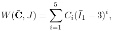 |
(6.27) |
where ![]() is the first invariant of the right deviatoric Cauchy Green
tensor and
is the first invariant of the right deviatoric Cauchy Green
tensor and ![]() are the material coefficients.
The material behavior is controlled by the following properties:
are the material coefficients.
The material behavior is controlled by the following properties:
| Property | Description | Default | Field | |
|---|---|---|---|---|
| C1 | first coefficient (shear modulus) | 150000 | ✓ | |
| C2 | second coefficient | 0 | ✓ | |
| C3 | third coefficient | 0 | ✓ | |
| C4 | fourth coefficient | 0 | ✓ | |
| C5 | fifth coefficient | 0 | ✓ | |
| bulkModulus | bulk modulus for incompressibility | 100000 | ✓ | |
| bulkPotential | incompressibility potential function |
QUADRATIC |
YeohMaterials can be created with the following constructors:
| YeohMaterial() |
Create with default properties. |
| YeohMaterial (double C1, double C2, double C3, double kappa) |
Create three term material with |
| YeohMaterial (double C1, double C2, double C3, double C4, double C5, double kappa) |
Create five term material with |
6.10.2.8 Arruda-Boyce material
ArrudaBoyceMaterial is an incompressible isotropic material that implements the Arruda-Boyce model [2]. Its strain energy density is given by
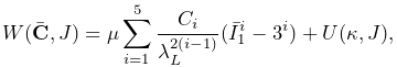 |
(6.27) |
where ![]() is the initial modulus,
is the initial modulus, ![]() the
locking stretch,
the
locking stretch, ![]() the first invariant of the
right deviatoric Cauchy Green tensor, and
the first invariant of the
right deviatoric Cauchy Green tensor, and
The material behavior is controlled by the following properties:
| Property | Description | Default | Field | |
|---|---|---|---|---|
| mu | initial modulus | 1000 | ✓ | |
| lambdaMax | locking stretch | 2.0 | ✓ | |
| bulkModulus | bulk modulus for incompressibility | 100000 | ✓ | |
| bulkPotential | incompressibility potential function |
QUADRATIC |
ArrudaBoyceMaterials can be created with the following constructors:
| ArrudaBoyceMaterial() |
Create with default properties. |
| ArrudaBoyceMaterial (double mu, double lmax, double kappa) |
Create with specified |
6.10.2.9 Veronda-Westmann material
VerondaWestmannMaterial is an incompressible isotropic material that implements the Veronda-Westmann model [28]. Its strain energy density is given by
| (6.28) |
where ![]() and
and ![]() are material coefficients and
are material coefficients and ![]() and
and
![]() the first and second invariants of the right deviatoric
Cauchy Green tensor.
the first and second invariants of the right deviatoric
Cauchy Green tensor.
The material behavior is controlled by the following properties:
| Property | Description | Default | Field | |
|---|---|---|---|---|
| C1 | first coefficient | 1000 | ✓ | |
| C2 | second coefficient | 10 | ✓ | |
| bulkModulus | bulk modulus for incompressibility | 100000 | ✓ | |
| bulkPotential | incompressibility potential function |
QUADRATIC |
VerondaWestmannMaterials can be created with the following constructors:
| VerondaWestmannMaterial() |
Create with default properties. |
| VerondaWestmannMaterial (double C1, double C2, double kappa) |
Create with specified |
6.10.2.10 Incompressible material
IncompressibleMaterial is an incompressible isotropic material that implements pure incompressibility, with an energy density function given by
| (6.28) |
Because it responds only to dilational strains, it must be used in conjunction with another material to resist deviatoric strains. In this context, it can be used to provide dilational support to deviatoric-only materials such as the FullBlemkerMuscle (Section 6.10.3.3).
The material behavior is controlled by the following properties:
| Property | Description | Default | Field | |
|---|---|---|---|---|
| bulkModulus | bulk modulus for incompressibility | 100000 | ✓ | |
| bulkPotential | incompressibility potential function |
QUADRATIC |
IncompressibleMaterials can be created with the following constructors:
| IncompressibleMaterial() |
Create with default values. |
| IncompressibleMaterial (double kappa) |
Create with specified |
6.10.3 Muscle materials
Muscle materials are used to exert stress along a particular direction within a material. This stress may contain both an active component, which depends on the muscle excitation, and a passive component, which depends solely on the stretch along the prescribed direction. Because most muscle materials act only along one direction, they are typically deployed within an FEM as additional materials that act in addition to an underlying material. This can be done using either muscle bundles within a FemMuscleModel (Section 6.9.1.1) or material bundles within any FEM model (Sections 6.8 and 7.5.2).
All of the muscle materials described below assume (near)
incompressibility, and so the directional stress is a function of the
deviatoric stretch ![]() along the muscle direction instead of the
overall stretch
along the muscle direction instead of the
overall stretch ![]() . The former can be determined from the
latter via
. The former can be determined from the
latter via
| (6.28) |
where ![]() is the determinant of the deformation gradient. The
directional Cauchy stress
is the determinant of the deformation gradient. The
directional Cauchy stress ![]() resulting from the material is
computed from
resulting from the material is
computed from
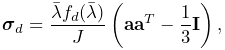 |
(6.29) |
where ![]() is a force term,
is a force term, ![]() is a unit vector indicating
the current muscle direction in spatial coordinates, and
is a unit vector indicating
the current muscle direction in spatial coordinates, and ![]() is the
is the ![]() identity matrix. In a purely passive case when the force arises
from a stress energy density function
identity matrix. In a purely passive case when the force arises
from a stress energy density function ![]() , we have
, we have
| (6.30) |
The muscle direction is specified in one of two ways, depending on how
the muscle material is deployed. All muscle materials export a
property restDir which specifies the direction in material
(rest) coordinates. It has a default value of ![]() , and can
be either set explicitly or bound to a field to allow it to vary over the
entire model (Section 7.5.2). However, if a muscle
material is deployed within a muscle bundle
(Section 6.9.1), then the restDir property is
ignored and the direction is instead specified by the
MuscleElementDesc components contained
within the bundle (Section 6.9.3).
, and can
be either set explicitly or bound to a field to allow it to vary over the
entire model (Section 7.5.2). However, if a muscle
material is deployed within a muscle bundle
(Section 6.9.1), then the restDir property is
ignored and the direction is instead specified by the
MuscleElementDesc components contained
within the bundle (Section 6.9.3).
Likewise, muscle excitation is specified using the material’s excitation property, unless the material is deployed within a muscle bundle, in which case it is controlled by the excitation property of the bundle.
6.10.3.1 Generic muscle
GenericMuscle
is a muscle material whose force term ![]() is given by
is given by
| (6.31) |
where ![]() is the excitation signal,
is the excitation signal, ![]() is a maximum stress
term, and
is a maximum stress
term, and ![]() is a passive force given by
is a passive force given by
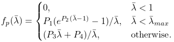 |
(6.32) |
In the equation above, ![]() is the exponential stress coefficient,
is the exponential stress coefficient,
![]() is the uncrimping factor, and
is the uncrimping factor, and ![]() and
and ![]() are computed to
provide
are computed to
provide ![]() continuity at
continuity at ![]() .
.
The material behavior is controlled by the following properties:
| Property | Description | Default | Field | |
|---|---|---|---|---|
| maxStress | maximum stress | 30000 | ✓ | |
| maxLambda |
|
1.4 | ✓ | |
| expStressCoeff | exponential stress coefficient | 0.05 | ✓ | |
| uncrimpingFactor | uncrimping factor | 6.6 | ✓ | |
| restDir | direction in material coordinates | ✓ | ||
| excitation | activation signal | 0 |
GenericMuscles can be created with the following constructors:
| GenericMuscle() |
Create with default values. |
| GenericMuscle (double maxLambda, double maxStress, double expStressCoef, double uncrimpFactor) |
Create with specified |
The constructors do not specify restDir. If the material is not being deployed within a muscle bundle, then restDir should also be set appropriately, either directly or via a field (Section 7.5.2).
6.10.3.2 Blemker muscle
BlemkerMuscle
is a muscle material implementing the directional component of the
model proposed by Sylvia Blemker [5]. Its force
term ![]() is given by
is given by
| (6.32) |
where ![]() is a maximum stress term,
is a maximum stress term, ![]() is the excitation
signal,
is the excitation
signal, ![]() is an active force-length curve, and
is an active force-length curve, and ![]() is
the passive force.
is
the passive force. ![]() and
and ![]() are described in
terms of
are described in
terms of ![]() :
:
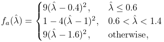 |
(6.33) |
and
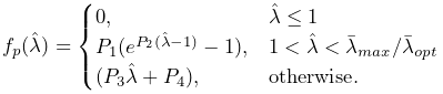 |
(6.34) |
In the equation for ![]() ,
, ![]() is the exponential stress
coefficient,
is the exponential stress
coefficient, ![]() is the uncrimping factor, and
is the uncrimping factor, and ![]() and
and ![]() are
computed to provide
are
computed to provide ![]() continuity at
continuity at ![]() .
.
The material behavior is controlled by the following properties:
| Property | Description | Default | Field | |
|---|---|---|---|---|
| maxStress | maximum stress | 300000 | ✓ | |
| optLambda |
|
1 | ✓ | |
| maxLambda |
|
1.4 | ✓ | |
| expStressCoeff | exponential stress coefficient | 0.05 | ✓ | |
| uncrimpingFactor | uncrimping factor | 6.6 | ✓ | |
| restDir | direction in material coordinates | ✓ | ||
| excitation | activation signal | 0 |
BlemkerMuscles can be created with the following constructors:
| BlemkerMuscle() |
Create with default values. |
| BlemkerMuscle (double maxLam, double optLam, double maxStress, double expStressCoef, double uncrimpFactor) |
Create with specified |
The constructors do not specify restDir. If the material is not being deployed within a muscle bundle, then restDir should also be set appropriately, either directly or via a field (Section 7.5.2).
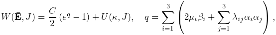
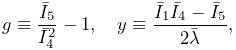
6.10.3.3 Full Blemker muscle
FullBlemkerMuscle
is a muscle material implementing the entire model proposed by Sylvia
Blemker [5]. This includes the directional
stress described in Section 6.10.3.2, plus additional
passive terms to model the tissue material matrix. The latter is based
on a strain energy density function ![]() given by
given by
| (6.34) |
where ![]() and
and ![]() are the along-fibre and cross-fibre
shear moduli, respectively, and
are the along-fibre and cross-fibre
shear moduli, respectively, and ![]() and
and ![]() are
Criscione invariants. The latter are defined as follows: Let
are
Criscione invariants. The latter are defined as follows: Let ![]() and
and ![]() be the invariants of the deviatoric left Cauchy
Green tensor
be the invariants of the deviatoric left Cauchy
Green tensor ![]() ,
, ![]() the unit vector giving the current muscle
direction in spatial coordinates, and
the unit vector giving the current muscle
direction in spatial coordinates, and ![]() and
and ![]() additional invariants defined by
additional invariants defined by
| (6.35) |
Then, defining
 |
![]() and
and ![]() are given by
are given by
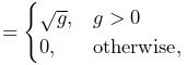 |
(6.36) | |||
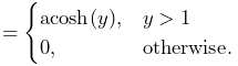 |
(6.37) |
At present, FullBlemkerMuscle does not implement a volumetric potential function
. That means it responds solely to deviatoric strains, and so if it is being used as a model’s primary material, it should be augmented with an additional material to provide resistance to compression. A simple choice for this is the purely incompressible material IncompressibleMaterial, described in Section 6.10.2.10.
The material behavior is controlled by the following properties:
| Property | Description | Default | Field | |
|---|---|---|---|---|
| maxStress | maximum stress | 300000 | ✓ | |
| optLambda |
|
1 | ✓ | |
| maxLambda |
|
1.4 | ✓ | |
| expStressCoeff | exponential stress coefficient | 0.05 | ✓ | |
| uncrimpingFactor | uncrimping factor | 6.6 | ✓ | |
| G1 | along-fibre shear modulus | 0 | ✓ | |
| G2 | cross-fibre shear modulus | 0 | ✓ | |
| restDir | direction in material coordinates | ✓ | ||
| excitation | activation signal | 0 |
FullBlemkerMuscles can be created with the following constructors:
| FullBlemkerMuscle() |
Create with default values. |
| BlemkerMuscle (double maxLam, double optLam, double maxStress, double expStressCoef, double uncrimpFactor, double G1, double G2) |
Create with |
The constructors do not specify restDir. If the material is not being deployed within a muscle bundle, then restDir should also be set appropriately, either directly or via a field (Section 7.5.2).
6.10.3.4 Simple force muscle
SimpleForceMuscle
is a very simple muscle material whose force term ![]() is
given by
is
given by
| (6.38) |
where ![]() is the excitation signal and
is the excitation signal and ![]() is a maximum
stress term. It can be useful as a debugging tool.
is a maximum
stress term. It can be useful as a debugging tool.
The material behavior is controlled by the following properties:
| Property | Description | Default | Field | |
|---|---|---|---|---|
| maxStress | maximum stress | 30000 | ✓ | |
| restDir | direction in material coordinates | ✓ | ||
| excitation | activation signal | 0 |
SimpleForceMuscles can be created with the following constructors:
| SimpleForceMuscle() |
Create with default values. |
| SimpleForceMuscle (double maxStress) |
Create with specified |
The constructors do not specify restDir. If the material is not being deployed within a muscle bundle, then restDir should also be set appropriately, either directly or via a field (Section 7.5.2).
![[LOGO]](data:image/png;base64,iVBORw0KGgoAAAANSUhEUgAAAAsAAAAOCAYAAAD5YeaVAAAAAXNSR0IArs4c6QAAAAZiS0dEAP8A/wD/oL2nkwAAAAlwSFlzAAALEwAACxMBAJqcGAAAAAd0SU1FB9wKExQZLWTEaOUAAAAddEVYdENvbW1lbnQAQ3JlYXRlZCB3aXRoIFRoZSBHSU1Q72QlbgAAAdpJREFUKM9tkL+L2nAARz9fPZNCKFapUn8kyI0e4iRHSR1Kb8ng0lJw6FYHFwv2LwhOpcWxTjeUunYqOmqd6hEoRDhtDWdA8ApRYsSUCDHNt5ul13vz4w0vWCgUnnEc975arX6ORqN3VqtVZbfbTQC4uEHANM3jSqXymFI6yWazP2KxWAXAL9zCUa1Wy2tXVxheKA9YNoR8Pt+aTqe4FVVVvz05O6MBhqUIBGk8Hn8HAOVy+T+XLJfLS4ZhTiRJgqIoVBRFIoric47jPnmeB1mW/9rr9ZpSSn3Lsmir1fJZlqWlUonKsvwWwD8ymc/nXwVBeLjf7xEKhdBut9Hr9WgmkyGEkJwsy5eHG5vN5g0AKIoCAEgkEkin0wQAfN9/cXPdheu6P33fBwB4ngcAcByHJpPJl+fn54mD3Gg0NrquXxeLRQAAwzAYj8cwTZPwPH9/sVg8PXweDAauqqr2cDjEer1GJBLBZDJBs9mE4zjwfZ85lAGg2+06hmGgXq+j3+/DsixYlgVN03a9Xu8jgCNCyIegIAgx13Vfd7vdu+FweG8YRkjXdWy329+dTgeSJD3ieZ7RNO0VAXAPwDEAO5VKndi2fWrb9jWl9Esul6PZbDY9Go1OZ7PZ9z/lyuD3OozU2wAAAABJRU5ErkJggg==)