ArtiSynth Modeling Guide
Last update: June, 2025
Contents
- Preface
- 1 ArtiSynth Overview
- 2 Supporting classes
-
3 Mechanical Models I
- 3.1 Points, particles, and springs
-
3.2 Rigid bodies
- 3.2.1 Frame markers
- 3.2.2 Example: a simple rigid body-spring model
- 3.2.3 Creating rigid bodies
- 3.2.4 Pose and velocity
- 3.2.5 Inertia and the surface mesh
- 3.2.6 Coordinate frames and the center of mass
- 3.2.7 Damping parameters
- 3.2.8 Rendering rigid bodies
- 3.2.9 Multiple meshes
- 3.2.10 Example: a composite rigid body
- 3.3 Mesh components
-
3.4 Joints and connectors
- 3.4.1 Joints and coordinate frames
- 3.4.2 Joint coordinates, constraints, and errors
- 3.4.3 Creating joints
- 3.4.4 Working with coordinates
- 3.4.5 Coordinate limits and locking
- 3.4.6 Example: a simple hinge joint
- 3.4.7 Joint coordinate handles
- 3.4.8 Constraint forces
- 3.4.9 Compliance and regularization
- 3.4.10 Example: an overconstrained linkage
- 3.4.11 Rendering joints
-
3.5 Joint components
- 3.5.1 Hinge joint
- 3.5.2 Slider joint
- 3.5.3 Cylindrical joint
- 3.5.4 Slotted hinge joint
- 3.5.5 Universal joint
- 3.5.6 Skewed universal joint
- 3.5.7 Gimbal joint
- 3.5.8 Spherical joint
- 3.5.9 Planar joint
- 3.5.10 Planar translation joint
- 3.5.11 Ellipsoid joint
- 3.5.12 Solid joint
- 3.5.13 Planar Connector
- 3.5.14 Segmented Planar Connector
- 3.5.15 Legacy Joints
- 3.5.16 Example: A multijointed arm
- 3.6 Setting joint coordinates
- 3.7 Frame springs
- 3.8 Other point-based forces
- 3.9 Attachments
- 3.10 Attached frames
-
4 Mechanical Models II
- 4.1 Simulation control properties
- 4.2 Units
- 4.3 Render properties
- 4.4 Custom rendering
- 4.5 Point-to-point muscles, tendons and ligaments
- 4.6 Distance Grids and Components
- 4.7 Transforming geometry
- 4.8 General component arrangements
- 4.9 Custom Joints
-
5 Simulation Control
- 5.1 Control Panels
- 5.2 Custom properties
- 5.3 Controllers and monitors
-
5.4 Probes
- 5.4.1 Numeric probe structure
- 5.4.2 Creating probes in code
- 5.4.3 Example: probes connected to SimpleMuscle
- 5.4.4 Data file format
- 5.4.5 Adding input probe data in code
- 5.4.6 Setting data from text or CSV files and other probes
- 5.4.7 Tracing probes
- 5.4.8 Position probes
- 5.4.9 Velocity probes
- 5.4.10 Example: controlling a point and frame
- 5.4.11 Numeric monitor probes
- 5.4.12 Numeric control probes
- 5.5 Working with TRC data
- 5.6 Application-Defined Menu Items
-
6 Finite Element Models
- 6.1 Overview
- 6.2 FEM model creation
- 6.3 FEM Geometry
-
6.4 Connecting FEM models to other components
- 6.4.1 Connecting nodes to rigid bodies or particles
- 6.4.2 Example: connecting a beam to a block
- 6.4.3 Connecting nodes directly to elements
- 6.4.4 Example: connecting two FEMs together
- 6.4.5 Finding which nodes to attach
- 6.4.6 Selecting nodes in the viewer
- 6.4.7 Example: two bodies connected by an FEM “spring”
- 6.4.8 Nodal-based attachments
- 6.4.9 Example: element vs. nodal-based attachments
- 6.5 FEM markers
- 6.6 Frame attachments
- 6.7 Incompressibility
- 6.8 Varying and augmenting material behaviors
- 6.9 Muscle activated FEM models
-
6.10 Material types
- 6.10.1 Linear
-
6.10.2 Hyperelastic materials
- 6.10.2.1 St Venant-Kirchoff material
- 6.10.2.2 Neo-Hookean material
- 6.10.2.3 Incompressible neo-Hookean material
- 6.10.2.4 Mooney-Rivlin material
- 6.10.2.5 Ogden material
- 6.10.2.6 Fung orthotropic material
- 6.10.2.7 Yeoh material
- 6.10.2.8 Arruda-Boyce material
- 6.10.2.9 Veronda-Westmann material
- 6.10.2.10 Incompressible material
- 6.10.3 Muscle materials
- 6.11 Stress, strain and strain energy
- 6.12 Rendering and Visualizations
- 7 Fields
- 8 Contact and Collision
- 9 Muscle Wrapping and Via Points
-
10 Inverse Simulation
- 10.1 Overview
-
10.2 Tracking controller components
- 10.2.1 Exciters
- 10.2.2 Motion targets
- 10.2.3 Regularization
- 10.2.4 Example: controlling ToyMuscleArm
- 10.2.5 Example: controlling an FEM muscle model
- 10.2.6 Force effector targets
- 10.2.7 Example: controlling tension in a spring
- 10.2.8 Target components
- 10.2.9 Point and frame exciters
- 10.2.10 Example: controlling ToyMuscleArm with FrameExciters
- 10.3 Tracking controller structure and settings
- 10.4 Managing probes and control panels
- 10.5 Inverse kinematics
- 10.6 Caveats and limitations
- 11 Skinning
- 12 Importing OpenSim Models
- 13 DICOM Images
- A Mathematical Review
Preface
This guide describes how to create mechanical and biomechanical models in ArtiSynth using its Java API. Detailed information on how to use the ArtiSynth GUI for model visualization, navigation and simulation control is given in the ArtiSynth User Interface Guide. It is also possible to interface ArtiSynth with, or run it under, MATLAB. For information on this, see the guide Interfacing ArtiSynth to MATLAB.
Information on how to install and configure ArtiSynth is given in the installation guides for Windows, MacOS, and Linux.
It is assumed that the reader is familiar with basic Java programming, including variable assignment, control flow, exceptions, functions and methods, object construction, inheritance, and method overloading. Some familiarity with the basic I/O classes defined in java.io.*, including input and output streams and the specification of file paths using File, as well as the collection classes ArrayList and LinkedList defined in java.util.*, is also assumed.
How to read this guide
Section 1 offers a general overview of ArtiSynth’s software design, and briefly describes the algorithms used for physical simulation (Section 1.2.3). The latter section may be skipped on first reading. A more comprehensive overview paper is available online.
The remainder of the manual gives detailed instructions on how to build various types of mechanical and biomechanical models. Sections 3 and 4 give detailed information about building general mechanical models, involving particles, springs, rigid bodies, joints, constraints, and contact. Section 5 describes how to add control panels, controllers, and input and output data streams to a simulation. Section 6 describes how to incorporate finite element models. The required mathematics is reviewed in Section A.
If time permits, the reader will profit from a top-to-bottom read. However, this may not always be necessary. Many of the sections contain detailed examples, all of which are available in the package artisynth.demos.tutorial and which may be run from ArtiSynth using Models > All demos > tutorial. More experienced readers may wish to find an appropriate example and then work backwards into the text and preceding sections for any needed explanatory detail.
Chapter 1 ArtiSynth Overview
ArtiSynth is an open-source, Java-based system for creating and simulating mechanical and biomechanical models, with specific capabilities for the combined simulation of rigid and deformable bodies, including finite element (FE) models, together with contact and constraints. It is presently directed at application domains in biomechanics, medicine, physiology, and dentistry, but it can also be applied to other areas such as traditional mechanical simulation, ergonomic design, and graphical and visual effects.
1.1 System structure
An ArtiSynth model is composed of a hierarchy of models and model components which are implemented by various Java classes. Components are broadly divided into simulation components, which include particles, rigid bodies, springs, connectors, force effectors, individual finite elements, constraints, etc., which are gathered together into models (including finite element models), and instrumentation components such as control panels, controllers and monitors, and input and output data streams (i.e., probes), which have the ability to control and record the simulation as it advances in time. Instrumentation components are presented in more detail in Chapter 5.
Every ArtiSynth component is an instance of ModelComponent, while components that contain subcomponents are instances of CompositeComponent. A ComponentList is a CompositeComponent which contains a list of other components of a specific type (such as particles, rigid bodies, springs, etc.).
All models and instrumentation components are collected together within a top-level container known as a root model. Simulation proceeds under the control of a scheduler, which advances the models through time using a physics simulator. A graphical user interface (GUI) allows users to view and edit the model hierarchy, modify component properties, and edit and temporally arrange the input and output probes using a timeline display.
1.1.1 Simulation components
Simulation components are those used to build a model or set of models to be simulated. They are roughly divided into the following categories:
- Dynamic components
-
Components, such as particles and rigid bodies, that contain position and velocity state, and possibly mass. At present, dynamic components consist of Point, Frame, and their subclasses. All dynamic components implement the Java interface DynamicComponent. - Force effectors
-
Components, such as springs or finite elements, that exert forces between dynamic components. All force effectors implement the Java interface ForceEffector. Dynamic components are themselves also instances of ForceEffector, since they can exert velocity-based damping forces on themselves. - Constrainers
-
Components that enforce constraints between dynamic components. All constrainers implement the Java interface Constrainer. - Attachments
-
Components that can attach one dynamic component to another (see Section 1.2.4). While attachments are in principle the same as constraints, they are implemented using a different approach. All attachment components implement the Java interface DynamicAttachment. - Markers
-
Subclasses of dynamic components which are always attached to other dynamic components and contain the relevant attachment component internally. All currently implemented markers are subclasses of Marker (attached points) and AttachedFrame (attached frames). - Visual components
-
Components that provide graphical representation but do not actually affect the simulation. Examples of these include mesh components that are not connected to rigid bodies or FE models, and other implementations of RenderableComponent that are used for visualization only. - Models
-
Composite components that agglomerate simulation components into a single entity that contains state and can be advanced through time via the methods initialize(t0) and advance(t0, t1, flags), as discussed further in Section 1.2.1. All models implement the Java interface Model. The primary model types used by ArtiSynth are MechModel (Section 1.1.2), which is the primary container for a single mechanical or biomechanical model, and RootModel (Section 1.1.4), which combines one or more models together with instrumentation components to form a loadable application model.
1.1.2 The MechModel
In most ArtiSynth applications, the simulation components used to construct the model are collected under a single MechModel. This is a Model component that may contain particles, rigid bodies, FE models, constraints, attachments, various force effectors, and possibly other MechModels. When a simulation is run, the model’s advance() method invokes a physics simulator that advances these components forward in time (Section 1.2.3).
For convenience each MechModel contains a number of predefined containers for different component types, including:
container name description component type particles 3 DOF particles dynamic points other 3 DOF points dynamic rigidBodies 6 DOF rigid bodies dynamic frames other 6 DOF frames dynamic frameMarkers points which are attached to frames marker axialSprings point-to-point springs force multiPointSprings point-based springs with multiple via points force frameSprings 6 DOF springs between frames force meshBodies 3D surface mesh objects visual connectors joint-type connectors between bodies constrainer constrainers general constraints constrainer forceEffectors general force-effectors force models FE models and other MechModels model attachments attachments between dynamic components attachment renderables renderable components (for visualization only) visual
Each of these is a child component of MechModel and is implemented as a ComponentList. Special methods are provided for adding and removing items from them. If not used, the containers will simply remain empty.
Applications are not required to use these containers, and may instead create any component containment structure that is appropriate, as described in Section 4.8.
1.1.3 Instrumentation components
Instrumentation components consist primarily of control panels, which provide the ability to interactively adjust properties of simulation components, and simulation agents, which are used to set inputs and monitor outputs as a simulation proceeds (Section 1.2.1). Both are described in detail in Chapter 5.
- Control panels
-
GUI components that an application can create to interactively edit property values of simulation components. They are described in Section 5.1. - Input probes
-
Simulation agents that provide streams of input data to control the simulation. Such data may include external force values, muscle excitation levels, and position or velocity data for dynamic components which are being controlled parametrically. Input probes work via an apply(t) method, which is called before each simulation step to determine the value of the input data for time t and (typically) use this to set property values of simulation components associated with the probe. They are described in more detail in Section 5.4. - Controllers
-
Simulation agents that perform computations, based on input probe data or the state of the model, that are used to control the simulation. As with input probes, computed quantities typically include external forces, excitation levels, and positions or velocities. Computations are performed by an apply(t0,t1) method that is called before the simulation step between time t0 and t1. Controllers are often custom-defined by the application, but predefined controllers (such as the inverse tracking controller described in Chapter 10) are also available. They are described in more detail in Section 5.3. - Monitors
-
Simulation agents that compute simulation results, based on the state of the model. These results can be directed to an output probe, saved to a specific file, or just printed to the application console. Monitors are generally used to compute quantities that are not explicitly available as properties within the simulation components. Computations are performed by an apply(t0,t1) method that is called after the simulation step between time t0 and t1. Monitors are typically custom-defined by the application, and are described in more detail in Section 5.3. - Output probes
-
Simulation agents that provide streams of output data to record the results of the simulation. Such data may correspond directly to simulation component properties, or to values computed by Monitors. Common output probe data includes reaction forces, contact pressures, and the position or velocity data for dynamic components. Output probes work via an apply(t) method, which is called after a simulation step to determine and store the data for simulation time t; typically this data is determined from property values of simulation components associated with the probe. Output probes are described in more detail in Section 5.4.
1.1.4 The RootModel
The top-level component in the hierarchy is the root model, which is an application-specific subclass of RootModel and which contains a list of simulation models, along with containers for instrumentation components used to control and interact with these models. The containers in RootModel include:
container name description models top-level simulation models of the component hierarchy inputProbes input data streams for controlling the simulation controllers functions for controlling the simulation monitors functions for observing the simulation outputProbes output data streams for observing the simulation controlPanels application defined control panels for property editing renderables renderable components (for visualization only)
Root models are created either by applications overriding the root model’s build() method, or by reading the model directly from a .art file (Section 1.5.3).
When a simulation is run, the root model’s advance(,,) method is used to advance the simulation forward by a single time step. This involves applying any input probes and controllers, calling the advance() method for each of the simulation models, and then applying any monitors and output probes (Section 1.2.1).
1.1.5 Component numbers, names and path names
Whenever a component is added to the component hierarchy, it is assigned a unique number relative to its parent; the parent and number can be obtained using the methods getParent() and getNumber(), respectively. Components may also be assigned a name (using setName()) which is then returned using getName().
A component’s number is not the same as its index. The index gives the component’s sequential list position within the parent, and is always in the range
, where
is the parent’s number of child components. While indices and numbers frequently are the same, they sometimes are not. For example, a component’s number is guaranteed to remain unchanged as long as it remains attached to its parent; this is different from its index, which will change if any preceding components are removed from the parent. For example, if we have a set of components with numbers
0 1 2 3 4 5and components 2 and 4 are then removed, the remaining components will have numbers
0 1 3 5whereas the indices will be 0 1 2 3. This consistency of numbers is why they are used to identify components.
The names and/or numbers of a component and its ancestors can be used to form a component path name. This path has a construction analogous to Unix file path names, with the ’/’ character acting as a separator. Absolute paths start with ’/’, which indicates the root model. Relative paths omit the leading ’/’ and can begin lower down in the hierarchy. A typical path name might be
/models/JawHyoidModel/axialSprings/lad
For nameless components in the path, their numbers can be used instead. Numbers can also be used for components that have names. Hence the path above could also be represented using only numbers, as in
/0/0/1/5
although this would most likely appear only in machine-generated output.
1.2 Simulation overview
An overview of the ArtiSynth simulation mechanism is given here. More details are given in [11] and in the related overview paper.
1.2.1 Model advancement
ArtiSynth simulation works by advancing models forward in time using a series of time steps, with a physics integrator updating positions, velocities and forces for all of the dynamic components over each step. The step size is usually fixed, but can vary between models and also over different time ranges, as described in more detail in the “Advancing Models in Time” section of the ArtiSynth Reference Manual.
Simulation happens under the control of a scheduler, which determines the next time to advance to and then advances the root model using its advance() method. In pseudo-code, this looks like:
Most often, the next advance time is determined by adding the value of the root model’s maxStepSize property to t0.
Within its advance() method, the root model in turn calls the advance() methods for its collection of models, while also calling the apply() methods for the model agents. For each model, the advancement sequence typically looks like that shown in Figure 1.1, with any input probes and controllers called before the advance() method and any monitors and output probes called after. The preadvance() method is an additional method that a model can use to perform pre-step initialization before input probes and controllers are called.
By default, the update interval ![]() in Figure 1.1 equals
the maxStepSize of the root model. However,
in Figure 1.1 equals
the maxStepSize of the root model. However, ![]() will be less if required
by the model’s own maxStepSize value, or a smaller (explicit) update
interval for any of the output probes. Figure 1.1 also
assumes that all of the model agents are explicitly associated with the
model. Input probes and controllers that are not associated with the
model will be applied before the preadvance() method, and monitors
and output probes not associated with the model will be called after those that
are. Again, more precise details on this are given in the “Advancing Models in
Time” section of the
ArtiSynth Reference Manual.
will be less if required
by the model’s own maxStepSize value, or a smaller (explicit) update
interval for any of the output probes. Figure 1.1 also
assumes that all of the model agents are explicitly associated with the
model. Input probes and controllers that are not associated with the
model will be applied before the preadvance() method, and monitors
and output probes not associated with the model will be called after those that
are. Again, more precise details on this are given in the “Advancing Models in
Time” section of the
ArtiSynth Reference Manual.
1.2.2 Full coordinate formulation
It is important to understand that ArtiSynth uses a full coordinate
formulation, in which the position and velocity of each dynamic body is both
represented and solved using full, or unconstrained, coordinates, with extra
equations added to the system solve to account for constraints such as joints
and contact. In particular, point positions and velocities are represented
using 3-vectors, while the “positions” of RigidBody and Frame
components are represented as the translation and orientation of their
coordinate frames. Internally, these frames are stored as a 3-vector plus a
quaternion, but they are most often presented to the application as the body’s
pose, which is the ![]() homogeneous transformation
homogeneous transformation ![]() that
maps points from body to world coordinates:
that
maps points from body to world coordinates:
Here ![]() is a
is a ![]() rotation matrix and
rotation matrix and ![]() is a 3-vector
giving the location of the frame origin in world coordinates. The “velocity”
of RigidBody and Frame components is the spatial velocity
is a 3-vector
giving the location of the frame origin in world coordinates. The “velocity”
of RigidBody and Frame components is the spatial velocity
where ![]() and
and ![]() give the coordinate frame’s translational and
angular velocity in world coordinates. See Sections A.2
and A.5 for more details.
give the coordinate frame’s translational and
angular velocity in world coordinates. See Sections A.2
and A.5 for more details.
In contrast, some other simulation systems, including OpenSim [7], use reduced coordinates, in which the system dynamics are formulated using a smaller set of coordinates (such as joint angles) that implicitly take the system’s constraints into account. For example, a two degree-of-freedom (DOF) double pendulum in ArtiSynth is described using 12 degrees of freedom (six for each of the two bodies), with 10 constraint equations added to reduce the net DOF to two, while in OpenSim, a double pendulum would be described using only its two joint angles.
Each methodology has its own advantages. Reduced formulations yield systems with fewer degrees of freedom and no constraint errors. On the other hand, full coordinates make it easier to combine and connect a wide range of components, including rigid bodies and FE models, and they also allow modeling of situations where constraints are compliant (i.e., soft) such that the bodies connected to them can assume arbitrary poses with respect to each other. The speed advantages of reduced coordinates are much less important in ArtiSynth, where the main performance bottleneck is usually the computational requirements of FE models.
1.2.3 Time stepping and integration physics
This section describes the mechanical simulation that takes place inside the
advance() method of MechModel. An integrator is used to advance the
model from time ![]() to time
to time ![]() , corresponding to a time step given by
, corresponding to a time step given by
![]() . Several integrators are available and may be selected via
the model’s integrator property. The ones discussed here are the
first order explicit integrator ConstrainedForwardEuler and
the first-order implicit integrator ConstrainedBackwardEuler (which
is the system default).
. Several integrators are available and may be selected via
the model’s integrator property. The ones discussed here are the
first order explicit integrator ConstrainedForwardEuler and
the first-order implicit integrator ConstrainedBackwardEuler (which
is the system default).
Let the positions, velocities, and forces associated with all the dynamic
components be denoted by the composite vectors ![]() ,
, ![]() , and
, and ![]() . In
addition, let the composite mass matrix be given by
. In
addition, let the composite mass matrix be given by ![]() . Newton’s second law
then gives
. Newton’s second law
then gives
| (1.1) |
where the ![]() term accounts for various “fictitious” forces.
term accounts for various “fictitious” forces.
Each integration step involves solving for
the velocities ![]() at time step
at time step ![]() given the velocities and forces
at step
given the velocities and forces
at step ![]() . One way to do this is to solve the expression
. One way to do this is to solve the expression
| (1.2) |
for ![]() , where
, where ![]() is the step size and
is the step size and
![]() . Given the updated velocities
. Given the updated velocities ![]() , one can
determine
, one can
determine ![]() from
from
| (1.3) |
where ![]() accounts for situations (such as rigid bodies) where
accounts for situations (such as rigid bodies) where
![]() , and then solve for the updated positions using
, and then solve for the updated positions using
| (1.4) |
(1.2) and (1.4) by themselves comprise a simple symplectic Euler integrator.
In addition to forces, bilateral and unilateral constraints give rise to (generally) nonlinear constraint equations of the form
| (1.5) |
Bilateral constraints are equality constraints that may include rigid body
joints, FEM incompressibility, and point-surface constraints, while unilateral
constraints are inequality constraints that include contact forces, friction
and joint limits. Linearizing (1.5) leads to locally linear
constraints on the velocity ![]() of the form
of the form
| (1.6) |
where ![]() and
and ![]() are the derivative matrices of
are the derivative matrices of ![]() . Because
. Because ![]() and
and
![]() are evaluated at step
are evaluated at step ![]() but generally vary in time, we can use their
time derivatives to improve constraint satisfaction for
but generally vary in time, we can use their
time derivatives to improve constraint satisfaction for ![]() by modifying
(1.6) to
by modifying
(1.6) to
| (1.7) |
where
| (1.8) |
Constraints give rise to constraint forces (in the directions ![]() and
and
![]() ) which supplement the forces of (1.1) in order to
enforce the constraint conditions. In addition, for unilateral constraints, we
have a complementarity condition in which
) which supplement the forces of (1.1) in order to
enforce the constraint conditions. In addition, for unilateral constraints, we
have a complementarity condition in which ![]() implies no constraint
force, and a constraint force implies
implies no constraint
force, and a constraint force implies ![]() . Any given constraint
usually involves only a few dynamic components and so
. Any given constraint
usually involves only a few dynamic components and so ![]() and
and ![]() are
generally sparse.
are
generally sparse.
Adding constraints to the velocity solve (1.2) leads to a mixed linear complementarity problem (MLCP) of the form
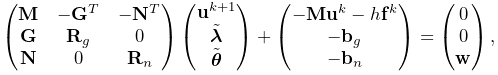 |
|||
| (1.9) |
where ![]() is a slack variable,
is a slack variable, ![]() and
and ![]() give the
constraint force impulses over the time step, and the constraint offsets
give the
constraint force impulses over the time step, and the constraint offsets ![]() and
and ![]() are typically set to
are typically set to ![]() and
and ![]() as per
(1.8).
as per
(1.8). ![]() and
and ![]() are optional diagonal regularization terms, which if non-zero serve to soften the constraints,
either to handle redundancy or to simulate physical compliance, as discussed
later in Sections 3.4.9
and 8.6.1. If
are optional diagonal regularization terms, which if non-zero serve to soften the constraints,
either to handle redundancy or to simulate physical compliance, as discussed
later in Sections 3.4.9
and 8.6.1. If ![]() or
or ![]() , then
, then ![]() or
or ![]() will typically also include a term related to the constraint error.
will typically also include a term related to the constraint error.
The actual constraint forces ![]() and
and ![]() can be determined by dividing
the constraint impulses by the time step
can be determined by dividing
the constraint impulses by the time step ![]() :
:
| (1.10) |
By itself, the MLCP (1.9) implements a constrained forward Euler integrator corresponding to setting the MechModel’s integrator property to ConstrainedForwardEuler.
For stiff systems, which often arise with systems containing FE models,
explicit integrators can be unstable unless the step size ![]() is set to a very
small value. This can typically be corrected by using an implicit
integrator. A first order example of this is a backward Euler integrator
in which
is set to a very
small value. This can typically be corrected by using an implicit
integrator. A first order example of this is a backward Euler integrator
in which ![]() is replaced with an approximation of
is replaced with an approximation of ![]() given by the
Taylor series expansion
given by the
Taylor series expansion
| (1.11) |
where ![]() and
and ![]() are the
negatives of the system stiffness and damping matrices,
respectively. Since
are the
negatives of the system stiffness and damping matrices,
respectively. Since
(1.11) can be reformulated as
| (1.12) |
which leads to the modified MLCP
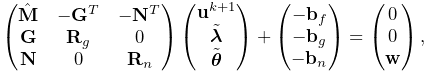 |
|||
| (1.13) |
where
The MLCP (1.13) corresponds to the default ArtiSynth integrator ConstrainedBackwardEuler. Higher order integrators, such as Newmark methods, often give rise to MLCPs with an equivalent form. Most ArtiSynth integrators use some variation of (1.13) to determine the system velocity at each time step; a description of the second order Trapezoidal integrator is given in [11].
To assemble (1.13), the MechModel component hierarchy is
traversed and the methods of the different component types are queried for the
required values. Dynamic components (type DynamicComponent) provide
![]() ,
, ![]() , and
, and ![]() ; force effectors (ForceEffector) determine
; force effectors (ForceEffector) determine ![]() and the stiffness/damping augmentation used to produce
and the stiffness/damping augmentation used to produce ![]() ; and constrainers
(Constrainer) supply
; and constrainers
(Constrainer) supply ![]() ,
, ![]() ,
, ![]() and
and ![]() .
.
1.2.4 Parametric and attached dynamic components
By default, a dynamic component is advanced through time in response to the forces applied to it. However, it is also possible to set a dynamic component to be parametric, such that it does not respond to forces and its position and/or velocity is either fixed or specified directly by the simulation. This is done by setting the component’s dynamic property to false, either through the GUI (by selecting the component(s) and choosing Edit properties ... from the context menu), or in code using the methods
| void setDynamic (boolean enable) |
Sets the dynamic property. |
| boolean isDynamic() |
Queries the dynamic property. |
Usage of setDynamic() is usually restricted to dynamic components that have mass, which include Particle and RigidBody but not Point or Frame.
Because the positions and velocities of parametric components are given, the MLCP (1.13) needs to be modified to reflect this. This involves partitioning the system velocity and force vectors into
where ![]() and
and ![]() denote the active (non-parametric) and parametric
components, respectively. The MLCP is then likewise partitioned. Considering
for simplicity the case with only bilateral constraints, this takes the form
denote the active (non-parametric) and parametric
components, respectively. The MLCP is then likewise partitioned. Considering
for simplicity the case with only bilateral constraints, this takes the form
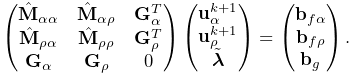 |
Since ![]() is given, the system can be reduced to
is given, the system can be reduced to
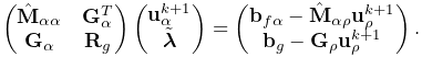 |
ArtiSynth also provides an attachment mechanism that allows dynamic components to be directly attached to other dynamic components. This is one of the primary means by which different parts of a model are connected together: points and particles (including FE nodes) can be attached to rigid bodies or other particles, and Frame components can be attached to other rigid bodies or connected to the nodes of an FE model.
When a dynamic component is attached, its position becomes a direct function of
the positions of the one or more master components to which it is
attached. For example, if a component ![]() is attached to a master component
is attached to a master component
![]() , then its position
, then its position ![]() is a function of the position
is a function of the position ![]() of
of ![]() :
:
Differentiating this yields a linear relationship between the velocities ![]() and
and ![]() of
of ![]() and
and ![]() ,
,
| (1.14) |
where ![]() is the derivative of
is the derivative of ![]() .
.
Attachments can be considered as constraints in which the positions/velocities of the attached components are constrained to be functions of the positions/velocities of the master components. While enforcement could be effected by adding velocity constraints of the form (1.14) to the system MLCP (1.13), in practice ArtiSynth actually uses the velocity constraints to preprocess the MLCP and remove the attached components from the system solve, which generally improves solve times. The attached positions/velocities are then updated after the solve based on the master positions/velocities.
As mentioned in Section 1.1.1, attachments are implemented by components which implement DynamicAttachment. These may be added to the model hierarchy separately, or, in the case of Marker and AttachedFrame components, embedded within specialized Point and Frame subclasses which are always attached.
Overall, a dynamic component can be in one of three states:
- active
-
Component is dynamic and unattached. The method isActive() returns true. The component will move in response to forces.
- parametric
-
Component is not dynamic, and is unattached. The method isParametric() returns true. The component will either remain fixed, or will move around in response to external inputs specifying the component’s position and/or velocity. One way to supply such inputs is to use controllers or input probes, as described in Section 5.
- attached
-
Component is attached. The method isAttached() returns true, and the method getAttachment() will return the actual attachment component. The component will move so as to follow the other master component(s) to which it is attached.
1.3 Basic packages
The core code of the ArtiSynth project is divided into three main packages, each with a number of sub-packages.
1.3.1 maspack
The packages under maspack contain general computational utilities that are independent of ArtiSynth and could be used in a variety of other contexts. The main packages are:
1.3.2 artisynth.core
The packages under artisynth.core contain the core code for ArtiSynth model components and its GUI infrastructure.
1.3.3 artisynth.demos
These packages contain demonstration models that illustrate ArtiSynth’s modeling capabilities:
1.4 Properties
ArtiSynth components expose properties, which provide a uniform interface for accessing their internal parameters and state. Properties vary from component to component; those for RigidBody include position, orientation, mass, and density, while those for AxialSpring include restLength and material. Properties are particularly useful for automatically creating control panels and probes, as described in Section 5. They are also used for automating component serialization.
Properties are described only briefly in this section; more detailed descriptions are available in the Maspack Reference Manual and the overview paper.
The set of properties defined for a component is fixed for that component’s class; while property values may vary between component instances, their definitions are class-specific. Properties are exported by a class through code contained in the class definition, as described in Section 5.2.
1.4.1 Querying and setting property values
Each property has a unique name that can be used to access its value interactively in the GUI. This can be done either by using a custom control panel (Section 5.1) or by selecting the component and choosing Edit properties ... from the right-click context menu).
Properties can also be accessed in code using their set/get accessor methods. Unless otherwise specified, the names for these are formed by simply prepending set or get to the property’s name. More specifically, a property with the name foo and a value type of Bar will usually have accessor signatures of
1.4.2 Property handles and paths
A property’s name can also be used to obtain a property handle through which its value may be queried or set generically. Property handles are implemented by the class Property and are returned by the component’s getProperty() method. getProperty() takes a property’s name and returns the corresponding handle. For example, components of type Muscle have a property excitation, for which a handle may be obtained using a code fragment such as
Property handles can also be obtained for subcomponents, using a property path that consists of a path to the subcomponent followed by a colon ‘:’ and the property name. For example, to obtain the excitation property for a subcomponent located by axialSprings/lad relative to a MechModel, one could use a call of the form
1.4.3 Composite and inheritable properties
Composite properties are possible, in which a property value is a composite object that in turn has subproperties. A good example of this is the RenderProps class, which is associated with the property renderProps for renderable objects and which itself can have a number of subproperties such as visible, faceStyle, faceColor, lineStyle, lineColor, etc.
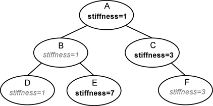
Properties can be declared to be inheritable, so that their values can be inherited from the same properties hosted by ancestor components further up the component hierarchy. Inheritable properties require a more elaborate declaration and are associated with a mode which may be either Explicit or Inherited. If a property’s mode is inherited, then its value is obtained from the closest ancestor exposing the same property whose mode is explicit. In Figure (1.2), the property stiffness is explicitly set in components A, C, and E, and inherited in B and D (which inherit from A) and F (which inherits from C).
1.5 Creating an application model
ArtiSynth applications are created by writing and compiling an application model that is a subclass of RootModel. This application-specific root model is then loaded and run by the ArtiSynth program.
The code for the application model should:
-
•
Declare a no-args constructor
-
•
Override the RootModel build() method to construct the application.
ArtiSynth can load a model either using the build method or by reading it from a file:
- Build method
-
ArtiSynth creates an instance of the model using the no-args constructor, assigns it a name (which is either user-specified or the simple name of the class), and then calls the build() method to perform the actual construction.
- Reading from a file
-
ArtiSynth creates an instance of the model using the no-args constructor, and then the model is named and constructed by reading the file.
The no-args constructor should perform whatever initialization is required in both cases, while the build() method takes the place of the file specification. Unless a model is originally created using a file specification (which is very tedious), the first time creation of a model will almost always entail using the build() method.
The general template for application model code looks like this:
Here, the model itself is called MyModel, and is defined in the (hypothetical) package artisynth.models.experimental (placing models in the super package artisynth.models is common practice but not necessary).
Note: The build() method was only introduced in ArtiSynth 3.1. Prior to that, application models were constructed using a constructor taking a String argument supplying the name of the model. This method of model construction still works but is deprecated.
1.5.1 Implementing the build() method
As mentioned above, the build() method is responsible for actual model construction. Many applications are built using a single top-level MechModel. Build methods for these may look like the following:
First, a MechModel is created (with the name "mech" in this example, although any name, or no name, may be given) and added to the list of models in the root model using the addModel() method. Subsequent code then creates and adds the components required by the MechModel, as described in Chapters 3, 4 and 6. The build() method also creates and adds to the root model any agents required by the application (controllers, probes, etc.), as described in Section 5.
Each of the MechModel component containers described in Section 1.1.2 is associated with a set of access methods that allow components to be added, queried, and removed. For example, for points, these include:
| void addPoint (Point p) |
Adds point p to the container. |
| boolean removePoint (Point p) |
Removes point p from the container. |
| void clearPoints() |
Removes all points. |
| PointList<Point> points() |
Returns the point container. |
A component container itself is iterable, and also supplies the methods size() and get(int i) that return the number of components and the
![]() -th component in the container. For example, the following code fragment
shows two ways to iterate through the points in the points container:
-th component in the container. For example, the following code fragment
shows two ways to iterate through the points in the points container:
While a component container also contains add() and remove() methods, it is generally recommended that these not be used for modifying the contents of the default containers.
Applications do not have to use the default component containers. Instead, they may create their own custom containers, as described in Section 4.8.
When constructing a model, there is no fixed order in which components need to be added. For instance, in the above example, addModel(mech) could be called near the end of the build() method rather than at the beginning. However, all components needed for the simulation must be added somewhere to the MechModel component hierarchy during the build process. This includes any components referenced by other components. For instance, an axial spring (Section 3.1) refers to two points. If either of these points have not been added to the hierarchy, an exception similar to the following will be raised after the build() method exits:
The build() method supplies a String array as an argument, which can be used to transmit application arguments in a manner analogous to the args argument passed to static main() methods. Build arguments can be specified when a model is loaded directly from a class using Models > Load from class ..., or when the startup model is set to automatically load a model when ArtiSynth is first started (Settings > Startup model). Details are given in the “Loading, Simulating and Saving Models” section of the User Interface Guide.
Build arguments can also be listed directly on the ArtiSynth command line when specifying a model to load using the -model <classname> option. This is done by enclosing the desired arguments within square brackets [ ] immediately following the -model option. So, for example,
> artisynth -model projects.MyModel [ -size 50 ]
would cause the strings "-size" and "50" to be passed to the build() method of MyModel.
1.5.2 Making models visible to ArtiSynth
In order to load an application model into ArtiSynth, the classes associated with its implementation must be made visible to ArtiSynth. This usually involves adding the top-level class folder associated with the application code to the classpath used by ArtiSynth.
The demonstration models referred to in this guide belong to the package artisynth.demos.tutorial and are already visible to ArtiSynth.
In most current ArtiSynth projects, classes are stored in a folder tree separate from the source code, with the top-level class folder named classes, located one level below the project root folder. A typical top-level class folder might be stored in a location like this:
/home/joeuser/artisynthProjects/classes
In the example shown in Section 1.5, the model was created in the package artisynth.models.experimental. Since Java classes are arranged in a folder structure that mirrors package names, with respect to the sample project folder shown above, the model class would be located in
/home/joeuser/artisynthProjects/classes/artisynth/models/experimental
At present there are three ways to make top-level class folders known to ArtiSynth:
- Add projects to your Eclipse launch configuration
-
If you are using the Eclipse IDE, then you can add the project in which are developing your model code to the launch configuration that you use to run ArtiSynth. Other IDEs will presumably provide similar functionality.
- Add the folders to the external classpath
-
You can explicitly add the class folders to ArtiSynth’s external classpath. The easiest way to do this is to select “Settings > External classpath ...” from the Settings menu, which will open an external classpath editor which lists all the classpath entries in a large panel on the left. (When ArtiSynth is first installed, the external classpath has no entries, and so this panel will be blank.) Class folders can then by added via the “Add class folder” button, and the classpath is saved using the Save button.
- Add the folders to your CLASSPATH environment variable
-
If you are running ArtiSynth from the command line, using the artisynth command (or artisynth.bat on Windows), then you can define a CLASSPATH environment variable in your environment and add the needed folders to this.
1.5.3 Loading and running a model
If a model’s classes are visible to ArtiSynth, then it may be loaded into ArtiSynth in several ways:
- Loading from the Model menu
-
If the root model is contained in a package located under artisynth.demos or artisynth.models, then it will appear in the default model menu (Models in the main menu bar) under the submenu All demos or All models.
- Loading by class path
-
A model may also be loaded by choosing “Load from class ...” from the Models menu and specifying its package name and then choosing its root model class. It is also possible to use the -model <classname> command line argument to have a model loaded directly into ArtiSynth when it starts up.
- Loading from a file
-
If a model has been saved to a .art file, it may be loaded from that file by choosing File > Load model ....
These methods are described in detail in the section “Loading and Simulating Models” of the ArtiSynth User Interface Guide.
The demonstration models referred to in this guide should already be present in the model menu and may be loaded from the submenu Models > All demos > tutorial.
Once a model is loaded, it can be simulated, or run. Simulation of the model can then be started, paused, single-stepped, or reset using the play controls (Figure 1.3) located at the upper right of the ArtiSynth window frame. Starting and stopping a simulation is done by clicking play/pause, while reset resets the simulation to time 0. The single-step button advances the simulation by one time step. The stop-all button will also stop the simulation, along with any Jython commands or scripts that are running.
Comprehensive information on exploring and interacting with models is given in the ArtiSynth User Interface Guide.
Chapter 2 Supporting classes
ArtiSynth uses a large number of supporting classes, mostly defined in the super package maspack, for handling mathematical and geometric quantities. Those that are referred to in this manual are summarized in this section.
2.1 Vectors and matrices
Among the most basic classes are those used to implement vectors and matrices, defined in maspack.matrix. All vector classes implement the interface Vector and all matrix classes implement Matrix, which provide a number of standard methods for setting and accessing values and reading and writing from I/O streams.
General sized vectors and matrices are implemented by VectorNd and MatrixNd. These provide all the usual methods for linear algebra operations such as addition, scaling, and multiplication:
As illustrated in the above example, vectors and matrices both provide a toString() method that allows their elements to be formatted using a C-printf style format string. This is useful for providing concise and uniformly formatted output, particularly for diagnostics. The output from the above example is
result= 4.000 12.000 12.000 24.000 20.000
Detailed specifications for the format string are provided in the documentation for NumberFormat.set(String). If either no format string, or the string "%g", is specified, toString() formats all numbers using the full-precision output provided by Double.toString(value).
For computational efficiency, a number of fixed-size vectors and matrices are also provided. The most commonly used are those defined for three dimensions, including Vector3d and Matrix3d:
2.2 Rotations and transformations
maspack.matrix contains a number of classes that implement rotation matrices, rigid transforms, and affine transforms.
Rotations (Section A.1) are commonly described using a RotationMatrix3d, which implements a rotation matrix and contains numerous methods for setting rotation values and transforming other quantities. Some of the more commonly used methods are:
Rotations can also be described by AxisAngle, which characterizes a rotation as a single rotation about a specific axis.
Rigid transforms (Section A.2) are used by ArtiSynth to describe a rigid body’s pose, as well as its relative position and orientation with respect to other bodies and coordinate frames. They are implemented by RigidTransform3d, which exposes its rotational and translational components directly through the fields R (a RotationMatrix3d) and p (a Vector3d). Rotational and translational values can be set and accessed directly through these fields. In addition, RigidTransform3d provides numerous methods, some of the more commonly used of which include:
Affine transforms (Section A.3) are used by ArtiSynth to effect scaling and shearing transformations on components. They are implemented by AffineTransform3d.
Rigid transformations are actually a specialized form of affine transformation in which the basic transform matrix equals a rotation. RigidTransform3d and AffineTransform3d hence both derive from the same base class AffineTransform3dBase.
2.3 Points and Vectors
The rotations and transforms described above can be used to transform both vectors and points in space.
Vectors are most commonly implemented using Vector3d, while points can be implemented using the subclass Point3d. The only difference between Vector3d and Point3d is that the former ignores the translational component of rigid and affine transforms; i.e., as described in Sections A.2 and A.3, a vector v has an implied homogeneous representation of
| (2.1) |
while the representation for a point p is
| (2.2) |
Both classes provide a number of methods for applying rotational and affine transforms. Those used for rotations are
where R is a rotation matrix and v1 is a vector (or a point in the case of Point3d).
The methods for applying rigid or affine transforms include:
where X is a rigid or affine transform. As described above, in the case of Vector3d, these methods ignore the translational part of the transform and apply only the matrix component (R for a RigidTransform3d and A for an AffineTransform3d). In particular, that means that for a RigidTransform3d given by X and a Vector3d given by v, the method calls
produce the same result.
2.4 Spatial vectors and inertias
The velocities, forces and inertias associated with 3D coordinate frames and rigid bodies are represented using the 6 DOF spatial quantities described in Sections A.5 and A.6. These are implemented by classes in the package maspack.spatialmotion.
Spatial velocities (or twists) are implemented by Twist, which exposes its translational and angular velocity components through the publicly accessible fields v and w, while spatial forces (or wrenches) are implemented by Wrench, which exposes its translational force and moment components through the publicly accessible fields f and m.
Both Twist and Wrench contain methods for algebraic operations such as addition and scaling. They also contain transform() methods for applying rotational and rigid transforms. The rotation methods simply transform each component by the supplied rotation matrix. The rigid transform methods, on the other hand, assume that the supplied argument represents a transform between two frames fixed within a rigid body, and transform the twist or wrench accordingly, using either (A.27) or (A.29).
The spatial inertia for a rigid body is implemented by SpatialInertia, which contains a number of methods for setting its value given various mass, center of mass, and inertia values, and querying the values of its components. It also contains methods for scaling and adding, transforming between coordinate systems, inversion, and multiplying by spatial vectors.
2.5 Meshes
ArtiSynth makes extensive use of 3D meshes, which are defined in maspack.geometry. They are used for a variety of purposes, including visualization, collision detection, and computing physical properties (such as inertia or stiffness variation within a finite element model).
A mesh is essentially a collection of vertices (i.e., points) that are topologically connected in some way. All meshes extend the abstract base class MeshBase, which supports the vertex definitions, while subclasses provide the topology.
Through MeshBase, all meshes provide methods for adding and accessing vertices. Some of these include:
Vertices are implemented by Vertex3d, which defines the position of the vertex (returned by the method getPosition()), and also contains support for topological connections. In addition, each vertex maintains an index, obtainable via getIndex(), that equals the index of its location within the mesh’s vertex list. This makes it easy to set up parallel array structures for augmenting mesh vertex properties.
Mesh subclasses currently include:
- PolygonalMesh
-
Implements a 2D surface mesh containing faces implemented using half-edges.
- PolylineMesh
-
Implements a mesh consisting of connected line-segments (polylines).
- PointMesh
-
Implements a point cloud with no topological connectivity.
PolygonalMesh is used quite extensively and provides a number of methods for implementing faces, including:
The class Face implements a face as a counter-clockwise arrangement of vertices linked together by half-edges (class HalfEdge). Face also supplies a face’s (outward facing) normal via getNormal().
Some mesh uses within ArtiSynth, such as collision detection, require a triangular mesh; i.e., one where all faces have three vertices. The method isTriangular() can be used to check for this. Meshes that are not triangular can be made triangular using triangulate().
2.5.1 Mesh creation
Meshes are most commonly created using either one of the factory methods supplied by MeshFactory, or by reading a definition from a file (Section 2.5.5). However, it is possible to create a mesh by direct construction. For example, the following code fragment creates a simple closed tetrahedral surface:
Some of the more commonly used factory methods for creating polyhedral meshes include:
Each factory method creates a mesh in some standard coordinate
frame. After creation, the mesh can be transformed using the
transform(X) method, where X is either a rigid transform (
RigidTransform3d) or a more general affine
transform (AffineTransform3d).
For example, to create a rotated box centered on ![]() ,
one could do:
,
one could do:
One can also scale a mesh using scale(s), where s is a single scale factor, or scale(sx,sy,sz), where sx, sy, and sz are separate scale factors for the x, y and z axes. This provides a useful way to create an ellipsoid:
MeshFactory can also be used to create new meshes by performing Boolean operations on existing ones:
2.5.2 Setting normals, colors, and textures
Meshes provide support for adding normal, color, and texture information, with the exact interpretation of these quantities depending upon the particular mesh subclass. Most commonly this information is used simply for rendering, but in some cases normal information might also be used for physical simulation.
For polygonal meshes, the normal information described here is used only for smooth shading. When flat shading is requested, normals are determined directly from the faces themselves.
Normal information can be set and queried using the following methods:
The method setNormals() takes two arguments: a set of normal vectors (nrmls), along with a set of index values (indices) that map these normals onto the vertices of each of the mesh’s geometric features. Often, there will be one unique normal per vertex, in which case nrmls will have a size equal to the number of vertices, but this is not always the case, as described below. Features for the different mesh subclasses are: faces for PolygonalMesh, polylines for PolylineMesh, and vertices for PointMesh. If indices is specified as null, then normals is assumed to have a size equal to the number of vertices, and an appropriate index set is created automatically using createVertexIndices() (described below). Otherwise, indices should have a size of equal to the number of features times the number of vertices per feature. For example, consider a PolygonalMesh consisting of two triangles formed from vertex indices (0, 1, 2) and (2, 1, 3), respectively. If normals are specified and there is one unique normal per vertex, then the normal indices are likely to be
[ 0 1 2 2 1 3 ]
As mentioned above, sometimes there may be more than one normal per vertex. This happens in cases when the same vertex uses different normals for different faces. In such situations, the size of the nrmls argument will exceed the number of vertices.
The method setNormals() makes internal copies of the specified normal and index information, and this information can be later read back using getNormals() and getNormalIndices(). The number of normals can be queried using numNormals(), and individual normals can be queried or set using getNormal(idx) and setNormal(idx,nrml). All normals and indices can be explicitly cleared using clearNormals().
Color and texture information can be set using analogous methods. For colors, we have
When specified as float[], colors are given as RGB or
RGBA values, in the range ![]() , with array lengths of 3 and 4,
respectively. The colors returned by
getColors() are always RGBA
values.
, with array lengths of 3 and 4,
respectively. The colors returned by
getColors() are always RGBA
values.
With colors, there may often be fewer colors than the number of vertices. For instance, we may have only two colors, indexed by 0 and 1, and want to use these to alternately color the mesh faces. Using the two-triangle example above, the color indices might then look like this:
[ 0 0 0 1 1 1 ]
Finally, for texture coordinates, we have
When specifying indices using setNormals, setColors, or setTextureCoords, it is common to use the same index set as that which associates vertices with features. For convenience, this index set can be created automatically using
Alternatively, we may sometimes want to create a index set that assigns the same attribute to each feature vertex. If there is one attribute per feature, the resulting index set is called a feature index set, and can be created using
If we have a mesh with three triangles and one color per triangle, the resulting feature index set would be
[ 0 0 0 1 1 1 2 2 2 ]
Note: when a mesh is modified by the addition of new features (such as faces for PolygonalMesh), all normal, color and texture information is cleared by default (with normal information being automatically recomputed on demand if automatic normal creation is enabled; see Section 2.5.3). When a mesh is modified by the removal of features, the index sets for normals, colors and textures are adjusted to account for the removal.
For colors, it is possible to request that a mesh explicitly maintain colors for either its vertices or features (Section 2.5.4). When this is done, colors will persist when vertices or features are added or removed, with default colors being automatically created as necessary.
Once normals, colors, or textures have been set, one may want to know which of these attributes are associated with the vertices of a specific feature. To know this, it is necessary to find that feature’s offset into the attribute’s index set. This offset information can be found using the array returned by
For example, the three normals associated with a triangle at index ti can be obtained using
Alternatively, one may use the convenience methods
which return the attribute values for the ![]() -th vertex of
the feature indexed by fidx.
-th vertex of
the feature indexed by fidx.
In general, the various get methods return references to internal storage information and so should not be modified. However, specific values within the lists returned by getNormals(), getColors(), or getTextureCoords() may be modified by the application. This may be necessary when attribute information changes as the simulation proceeds. Alternatively, one may use methods such as setNormal(idx,nrml) setColor(idx,color), or setTextureCoords(idx,coords).
Also, in some situations, particularly with colors and textures, it may be desirable to not have color or texture information defined for certain features. In such cases, the corresponding index information can be specified as -1, and the getNormal(), getColor() and getTexture() methods will return null for the features in question.
2.5.3 Automatic creation of normals and hard edges
For some mesh subclasses, if normals are not explicitly set, they are computed automatically whenever getNormals() or getNormalIndices() is called. Whether or not this is true for a particular mesh can be queried by the method
Setting normals explicitly, using a call to setNormals(nrmls,indices), will overwrite any existing normal information, automatically computed or otherwise. The method
will return true if normals have been explicitly set, and false if they have been automatically computed or if there is currently no normal information. To explicitly remove normals from a mesh which has automatic normal generation, one may call setNormals() with the nrmls argument set to null.
More detailed control over how normals are automatically created may be available for specific mesh subclasses. For example, PolygonalMesh allows normals to be created with multiple normals per vertex, for vertices that are associated with either open or hard edges. This ability can be controlled using the methods
Having multiple normals means that even with smooth shading, open or hard edges will still appear sharp. To make an edge hard within a PolygonalMesh, one may use the methods
which control the hardness of edges between individual vertices, specified either directly or using their indices.
2.5.4 Vertex and feature coloring
The method setColors() makes it possible to assign any desired coloring scheme to a mesh. However, it does require that the user explicitly reset the color information whenever new features are added.
For convenience, an application can also request that a mesh explicitly maintain colors for either its vertices or features. These colors will then be maintained when vertices or features are added or removed, with default colors being automatically created as necessary.
Vertex-based coloring can be requested with the method
This will create a separate (default) color for each of the mesh’s vertices, and set the color indices to be equal to the vertex indices, which is equivalent to the call
where colors contains a default color for each vertex. However, once vertex coloring is enabled, the color and index sets will be updated whenever vertices or features are added or removed. Meanwhile, applications can query or set the colors for any vertex using getColor(idx), or any of the various setColor methods. Whether or not vertex coloring is enabled can be queried using
Once vertex coloring is established, the application will typically want to set the colors for all vertices, perhaps using a code fragment like this:
Similarly, feature-based coloring can be requested using the method
This will create a separate (default) color for each of the mesh’s features (faces for PolygonalMesh, polylines for PolylineMesh, etc.), and set the color indices to equal the feature index set, which is equivalent to the call
where colors contains a default color for each feature. Applications can query or set the colors for any vertex using getColor(idx), or any of the various setColor methods. Whether or not feature coloring is enabled can be queried using
2.5.5 Reading and writing mesh files
PolygonalMesh, PolylineMesh, and PointMesh all provide constructors that allow them to be created from a definition file, with the file format being inferred from the file name suffix:
| Suffix | Format | PolygonalMesh | PolylineMesh | PointMesh |
|---|---|---|---|---|
| .obj | Alias Wavefront | X | X | X |
| .ply | Polygon file format | X | X | |
| .stl | STereoLithography | X | ||
| .gts | GNU triangulated surface | X | ||
| .off | Object file format | X | ||
| .vtk | VTK ascii format | X | ||
| .vtp | VTK XML format | X | X |
The currently supported file formats, and their applicability to the different mesh types, are given in Table 2.1. For example, a PolygonalMesh can be read from either an Alias Wavefront .obj file or an .stl file, as show in the following example:
The file-based mesh constructors may throw an I/O exception if an I/O error occurs or if the indicated format does not support the mesh type. This exception must either be caught, as in the example above, or thrown out of the calling routine.
In addition to file-based constructors, all mesh types implement read and write methods that allow a mesh to be read from or written to a file, with the file format again inferred from the file name suffix:
For the latter methods, the argument zeroIndexed specifies zero-based vertex indexing in the case of Alias Wavefront .obj files, while fmtStr is a C-style format string specifying the precision and style with which the vertex coordinates should be written. (In the former methods, zero-based indexing is false and vertices are written using full precision.)
As an example, the following code fragment writes a mesh as an .stl file:
Sometimes, more explicit control is needed when reading or writing a mesh from/to a given file format. The constructors and read/write methods described above make use of a specific set of reader and writer classes located in the package maspack.geometry.io. These can be used directly to provide more explicit read/write control. The readers and writers (if implemented) associated with the different formats are given in Table 2.2.
| Suffix | Format | Reader class | Writer class |
|---|---|---|---|
| .obj | Alias Wavefront | WavefrontReader | WavefrontWriter |
| .ply | Polygon file format | PlyReader | PlyWriter |
| .stl | STereoLithography | StlReader | StlWriter |
| .gts | GNU triangulated surface | GtsReader | GtsWriter |
| .off | Object file format | OffReader | OffWriter |
| .vtk | VTK ascii format | VtkAsciiReader | |
| .vtp | VTK XML format | VtkXmlReader |
The general usage pattern for these classes is to construct the desired reader or writer with a path to the desired file, and then call readMesh() or writeMesh() as appropriate:
Both readMesh() and writeMesh() may throw I/O exceptions, which must be either caught, as in the example above, or thrown out of the calling routine.
For convenience, one can also use the classes GenericMeshReader or GenericMeshWriter, which internally create an appropriate reader or writer based on the file extension. This enables the writing of code that does not depend on the file format:
Here, fileName can refer to a mesh of any format supported by GenericMeshReader. Note that the mesh returned by readMesh() is explicitly cast to PolygonalMesh. This is because readMesh() returns the superclass MeshBase, since the default mesh created for some file formats may be different from PolygonalMesh.
2.5.6 Reading and writing normal and texture information
When writing a mesh out to a file, normal and texture information are also written if they have been explicitly set and the file format supports it. In addition, by default, automatically generated normal information will also be written if it relies on information (such as hard edges) that can’t be reconstructed from the stored file information.
Whether or not normal information will be written is returned by the method
This will always return true if any of the conditions described above have been met. So for example, if a PolygonalMesh contains hard edges, and multiple automatic normals are enabled (i.e., getMultipleAutoNormals() returns true), then getWriteNormals() will return true.
Default normal writing behavior can be overridden within the MeshWriter classes using the following methods:
where enable should be one of the following values:
- 0
-
normals will never be written;
- 1
-
normals will always be written;
- -1
-
normals will be written according to the default behavior described above.
When reading a PolygonalMesh from a file, if the file contains normal information with multiple normals per vertex that suggests the existence of hard edges, then the corresponding edges are set to be hard within the mesh.
2.5.7 Constructive solid geometry
ArtiSynth contains primitives for performing constructive solid geometry (CSG) operations on volumes bounded by triangular meshes. The class that performs these operations is maspack.collision.SurfaceMeshIntersector, and it works by robustly determining the intersection contour(s) between a pair of meshes, and then using these to compute the triangles that need to be added or removed to produce the necessary CSG surface.
The CSG operations include union, intersection, and difference, and are implemented by the following methods of SurfaceMeshIntersector:
Each takes two PolygonalMesh objects, mesh0 and mesh1, and creates and returns another PolygonalMesh which represents the boundary surface of the requested operation. If the result of the operation is null, the returned mesh will be empty.
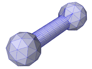
The example below uses findUnion to create a dumbbell shaped mesh from two balls and a cylinder:
The balls and cylinder are created using the MeshFactory methods createIcosahedralSphere() and createCylinder(), where the latter takes arguments ns, nr, and nh giving the number of slices along the circumference, the number of radial segments on each end cap, and the number of height segments along the length. The final resulting mesh is shown in Figure 2.1.
2.6 Reading source relative files
ArtiSynth applications frequently need to read in various kinds of data files, including mesh files (as discussed in Section 2.5.5), FEM mesh geometry (Section 6.2.2), probe data (Section 5.4.4), and custom application data.
Often these data files do not reside in an absolute location but instead in a location relative to the application’s class or source files. For example, it is common for applications to store geometric data in a subdirectory "geometry" located beneath the source directory. In order to access such files in a robust way, and ensure that the code does not break when the source tree is moved, it is useful to determine the application’s source (or class) directory at run time. ArtiSynth supplies several ways to conveniently handle this situation. First, the RootModel itself supplies the following methods:
The first method returns the path to the source directory of the root model, while the second returns the path to a file specified relative to the root model source directory. If the root model source directory cannot be found (see discussion at the end of this section) both methods return null. As a specific usage example, assume that we have an application model whose build() method needs to load in a mesh torus.obj from a subdirectory meshes located beneath the source directory. This could be done as follows:
A more general path finding utility is provided by maspack.util.PathFinder, which provides several static methods for locating source and class directories:
The “find” methods return a string path to the indicated class or source directory, while the “relative path” methods locate the class or source directory and append the additional path relpath. For all of these, the class is determined from classObj, either directly (if it is an instance of Class), by name (if it is a String), or otherwise by calling classObj.getClass(). When identifying a package by name, the name should be either a fully qualified class name, or a simple name that can be located with respect to the packages obtained via Package.getPackages(). For example, if we have a class whose fully qualified name is artisynth.models.test.Foo, then the following calls should all return the same result:
If the source directory for Foo happens to be /home/projects/src/artisynth/models/test, then
will return /home/projects/src/artisynth/models/test/geometry/mesh.obj.
When calling PathFinder methods from within the relevant class, one can specify this as the classObj argument.
With respect to the above example locating the file "meshes/torus.obj", the call to the root model method getSourceRelativePath() could be replaced with
Since this is assumed to be called from the root model’s build method, the “class” can be indicated by simply passing this to getSourceRelativePath().
As an alternative to placing data files in the source directory, one could place them in the class directory, and then use findClassDir() and getClassRelativePath(). If the data files were originally defined in the source directory, it will be necessary to copy them to the class directory. Some Java IDEs will perform this automatically.
The PathFinder methods work by climbing the class’s resource hierarchy. Source directories are assumed to be located relative to the parent of the root class directory, via one of the paths specified by getSourceRootPaths(). By default, this list includes "src", "source", and "bin". Additional paths can be added using addSourceRootPath(path), or the entire list can be set using setSourceRootPaths(paths).
At present, source directories will not be found if the reference class is contained in a jar file.
2.7 Reading and caching remote files
ArtiSynth applications often require the use of large data files to specify items such as FEM mesh geometry, surface mesh geometry, or medical imaging data. The size of these files may make it inconvenient to store them in any version control system that is used to store the application source code. As an alternative, ArtiSynth provides a file manager utility that allows such files to be stored on a separate server, and then downloaded on-demand and cached locally. To use this, one starts by creating an instance of a FileManager, using the constructor
where downloadPath is a path to the local directory where the downloaded file should be placed, and remoteSourceName is a URI indicating the remote server location of the files. After the file manager has been created, it can be used to fetch remote files and cache them locally, using various get methods:
Both of these look for the file destName specified relative to the local directory, and return a File handle for it if it is present. Otherwise, they attempt to download the file from the remote source location, place it in the local directory, and return a File handle for it. The location of the remote file is given relative to the remote source URI by destName for the first method and sourceName for the second.
A simple example of using a file manager within a RootModel build() method is given by the following fragment:
Here, a file manager is created that uses a local directory "geometry", located relative to the RootModel source directory (see Section 2.6), and looks for missing files relative to the URI
http://myserver.org/artisynth/data/geometry
The get() method is then used to obtain the file "tibia.obj" from the local directory. If it is not already present, it is downloaded from the remote location.
The FileManager contains other features and functionality, and one should consult its API documentation for more information.
Chapter 3 Mechanical Models I
This section details how to build basic multibody-type mechanical models consisting of particles, springs, rigid bodies, joints, and other constraints. Most of the ArtiSynth components described here are contained in the packages
artisynth.core.modelbase artisynth.core.mechmodels artisynth.core.materials
3.1 Points, particles, and springs
One of the most basic types of mechanical model consists simply of springs acting on points or particles.
3.1.1 Points
Points and particles are both instances of the class Point, and are dynamic components containing a three-dimensional position state and a corresponding velocity state. Subclasses of Point include Particle (discussed below), as well as markers (such as FrameMarker and FemMarker), which are massless point markers that can be attached to rigid bodies and FE models. The position and velocity state can be accessed by the following methods:
| Point3d getPosition() |
Returns the point’s position. |
| void setPosition (Point3d pos) |
Sets the point’s position. |
| Vector3d getVelocity() |
Returns the point’s velocity. |
| void setVelocity (Vector3d vel) |
Sets the point’s velocity. |
Points also maintain forces, which cause them and/or other dynamic components in the system to move. Force accessors include:
| Vector3d getForce() |
Returns the net force on the point. |
| Vector3d addForce(Vector3d f) |
Adds f to the point’s net force. |
| Vector3d getExternalForce() |
Returns the external force acting on the point. |
| void setExternalForce (Vector3d f) |
Sets the external force acting on the point to f. |
External forces are forces explicitly set by the application; once set, they will remain the same until setExternalForce() is called again. Net forces are the sum of the external forces plus all other forces arising from gravity, damping, springs, FE elements, etc. Net forces are zeroed and recomputed at the start of each simulation step. Applications (and custom defined force effectors in particular) can add to the net force using addForce().
3.1.2 Particles
Particles, implemented by Particle, are points that contain mass and hence can move and respond to forces independently. A subclass of Particle is FemNode3d, which describes the nodes of an FE model (Chapter 6).
Several constructors are available to create particles, including
| Particle (double mass) |
Create a particle with specified mass. |
| Particle (double mass, Point3d pos) |
Create a particle at a specified position. |
| Particle (double mass, double x, double y, double z) |
Create a particle at a specified position. |
| Particle (String name, double mass, double x, double y, double z) |
Create a named particle. |
Once created, a particle should be added to the MechModel. The standard way is to add it to the model’s particles container, as illustrated by the following code fragment:
The particles container can be managed by the following MechModel methods:
| void addParticle (Particle p) |
Adds particle p to the container. |
| boolean removeParticle (Particle p) |
Removes particle p from the container. |
| void clearParticles() |
Removes all particles. |
| PointList<Particle> particles() |
Returns the particles container. |
If desired, applications can also place particles in custom containers (Section 4.8).
3.1.3 Axial springs and materials
An axial spring is a simple spring that connects two points and is
implemented by the class
AxialSpring. This is a force effector component that exerts equal and opposite forces on the
two points, along the line separating them, with a magnitude ![]() that
is a function
that
is a function ![]() of the distance
of the distance ![]() between the points,
and the distance derivative
between the points,
and the distance derivative ![]() .
.
Axial springs connect only two points, but the more complex MultiPointSpring described in Chapter 9 can be used for more complex paths that contain via points and obstacle wrapping.
Each axial spring is associated with an axial material,
implemented by a subclass of
AxialMaterial, that specifies
the function ![]() . The most basic type of axial material is
a LinearAxialMaterial, which
determines
. The most basic type of axial material is
a LinearAxialMaterial, which
determines ![]() according to the linear relationship
according to the linear relationship
| (3.0) |
where ![]() is the rest length and
is the rest length and ![]() and
and ![]() are the stiffness and
damping terms. Both
are the stiffness and
damping terms. Both ![]() and
and ![]() are properties of the material, while
are properties of the material, while
![]() is a property of the spring.
is a property of the spring.
Axial springs are assigned a linear axial material by default. More complex, nonlinear axial materials may be defined in the package artisynth.core.materials. Setting or querying a spring’s material may be done with the methods setMaterial() and getMaterial().
3.1.4 Axial spring components
Constructors that create an AxialSpring include:
| AxialSpring (double k, double d, double l0) |
Create a spring with a linear material. |
| AxialSpring (String name, double k, double d, double l0) |
Create a named spring with a linear material. |
| AxialSpring (String name, double l0) |
Create a named spring with specified rest length. |
| AxialSpring (String name) |
Create a named spring. |
All of these create springs with linear axial material, with the parameters
k, d, and l0 specifying stiffness, damping, and rest
length. If not specified, these have default value of ![]() ,
, ![]() and
and ![]() .
.
If a different axial material is needed (Section 3.1.7), the following methods can be used to query and set the material:
| AxialMaterial getMaterial() |
Returns the current material. |
| void setMaterial (AxialMaterial mat) |
Sets the current material. |
Once created, an axial spring must be connected to its points and added to the MechModel. The following methods can be used to connect the points:
| void setPoints (Point p0, Point p1) |
Attaches the spring to points p0 and p1. |
| void setPoints (Point p0, Point p1, double l0) |
Attaches p0 and p1 and sets the rest length. |
The standard way to add a spring to the MechModel is to use the model’s axialSprings container, which is managed using the following MechModel methods:
| void addAxialSpring (AxialSpring spr) |
Adds spring spr to the container. |
| boolean removeAxialSpring (AxialSpring spr) |
Removes spring spr from the container. |
| void clearAxialSprings() |
Removes all springs. |
| RenderableComponentList<AxialSpring> axialSprings() |
Returns the axialSprings container. |
If desired, applications can also place springs in custom containers (Section 4.8).
MechModel also supplies a convenience method to both connect the points and add the spring to the model (the points themselves must still be added separately):
| void attachAxialSpring (Point p0, Point p1, AxialSpring spr) |
Attaches spr to p0 and p1 and adds it to the model. |
3.1.5 Example: a simple particle-spring model
A complete application model that implements a simple particle-spring model is given below.
Line 1 of the source defines the package in which the model class will reside, in this case artisynth.demos.tutorial. Lines 3-8 import definitions for other classes that will be used.
The model application class is named ParticleSpring and declared to extend RootModel (line 13), and the build() method definition begins at line 15. (A no-args constructor is also needed, but because no other constructors are defined, the compiler creates one automatically.)
To begin, the build() method creates a MechModel named "mech", and then adds it to the models list of the root model using the addModel() method (lines 18-19). Next, two particles, p1 and p2, are created, with masses equal to 2 and initial positions at 0, 0, 0, and 1, 0, 0, respectively (lines 22-23). Then an axial spring is created, with end points set to p1 and p2, and assigned a linear material with a stiffness and damping of 20 and 10 (lines 24-27). Finally, after the particles and the spring are created, they are added to the particles and axialSprings lists of the MechModel using the methods addParticle() and addAxialSpring() (lines 30-32).
At this point in the code, both particles are defined to be
dynamically controlled, so that running the simulation would cause
both to fall under the MechModel’s default gravity acceleration
of ![]() . However, for this example, we want the first
particle to remain fixed in place, so we set it to be non-dynamic (line 34), meaning that the physical simulation will not
update its position in response to forces (Section
1.2.4).
. However, for this example, we want the first
particle to remain fixed in place, so we set it to be non-dynamic (line 34), meaning that the physical simulation will not
update its position in response to forces (Section
1.2.4).
The remaining calls control aspects of how the model is graphically rendered. setBounds() (line 37) increases the model’s “bounding box” so that by default it will occupy a larger part of the viewer frustum. The convenience method RenderProps.setSphericalPoints() is used to set points p1 and p2 to render as solid red spheres with a radius of 0.06, while RenderProps.setCylindricalLines() is used to set spring to render as a solid blue cylinder with a radius of 0.02. More details about setting render properties are given in Section 4.3.
3.1.6 Damping parameters
Mechanical models usually contain damping forces in addition to spring-type restorative forces. Damping generates forces that reduce dynamic component velocities, and is usually the major source of energy dissipation in the model. Damping forces can be generated by the spring components themselves, as described above.
A general damping can be set for all particles by setting the MechModel’s pointDamping property. This causes a force
| (3.0) |
to be applied to all particles, where ![]() is the value of the pointDamping and
is the value of the pointDamping and ![]() is the particle’s velocity.
is the particle’s velocity.
pointDamping can be set and queried using the MechModel methods
In general, whenever a component has a property propX, that property can be set and queried in code using methods of the form
setPropX (T d); T getPropX();where T is the type associated with the property.
pointDamping can also be set for particles individually. This property is inherited (Section 1.4.3), so that if not set explicitly, it inherits the nearest explicitly set value in an ancestor component.
3.1.7 Axial materials
As indicated above, different materials can be supplied to an axial spring in addition to the default linear material. Most of these are related to modeling muscles, tendons and ligaments and are presented in detail in Section 4.5.
Application authors may also create their own custom axial materials by subclassing AxialMaterial and overriding the functions
| double computeF (double l, double ldot, double l0, double excitation) |
Computes tension |
| double computeDFdl (double l, double ldot, double l0, double excitation) |
Computes |
| double computeDFdldot (double l, double ldot, double l0, double excitation) |
Computes |
| boolean isDFdldotZero() |
Returns true if |
where l and l0 are the muscle length and rest length, ldot is
![]() , and excitation is an additional excitation signal
, and excitation is an additional excitation signal ![]() ,
which is usually in the range
,
which is usually in the range ![]() and is used to implement active springs
and in particular is used to implement the muscle materials of
Section 4.5.
and is used to implement active springs
and in particular is used to implement the muscle materials of
Section 4.5.
The first three methods should return the values of
| (3.0) |
respectively, while the last method should return true if
![]() ; i.e., it is
always 0.
; i.e., it is
always 0.
3.2 Rigid bodies
Rigid bodies are implemented in ArtiSynth by the class RigidBody, which is a dynamic component containing a six-dimensional position and orientation state, a corresponding velocity state, an inertia, and an optional surface mesh.
A rigid body is associated with its own 3D spatial coordinate frame, and is a subclass of the more general Frame component. The combined position and orientation of this frame with respect to world coordinates defines the body’s pose, and the associated 6 degrees of freedom describe its “position” state.
3.2.1 Frame markers
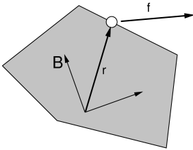
ArtiSynth makes extensive use of markers, which are (massless) points attached to dynamic components in the model. Markers are used for graphical display, implementing attachments, and transmitting forces back onto the underlying dynamic components.
Frame markers are markers that can be attached to a Frame (which includes RigidBody as a subclass), as illustrated in Figure 3.2. They are frequently used to provide the anchor points for attaching springs and, more generally, applying forces to the body.
Frame markers are implemented by the class FrameMarker, which is a subclass of Point. The methods
| Point3d getLocation () | |
| void setLocation (Point3d r) |
get and set the marker’s location ![]() with respect to the frame’s
coordinate system. When a 3D force
with respect to the frame’s
coordinate system. When a 3D force ![]() is applied to the marker, it
generates a spatial force
is applied to the marker, it
generates a spatial force ![]() (Section
A.5) on the frame given by
(Section
A.5) on the frame given by
| (3.0) |
Frame markers can be created using a variety of constructors, including
| FrameMarker () | |
| FrameMarker (String name) | |
| FrameMarker (Frame frame, Point3d loc) |
where FrameMarker() creates an empty marker, FrameMarker(name) creates an empty marker with a name, and FrameMarker(frame,loc) creates an unnamed marker attached to frame at the location loc with respect to the frame’s coordinates. A marker’s frame can also be queried and set with the methods
| void setFrame (Frame frame) | |
| Frame getFrame () |
Once created, a frame marker must be added to the MechModel. This can be done by adding it to the MechModel’s frameMarkers container, which is managed using the following MechModel methods:
| void addFrameMarker (FrameMarker m) |
Adds marker m to the container. |
| void addFrameMarker (FrameMarker m, Frame frame, Point3d loc) |
Adds m and sets its frame and location. |
| boolean removeFrameMarker (FrameMarker m) |
Removes marker m from the container. |
| void clearFrameMarkers() |
Removes all markers. |
| PointList<FrameMarker> frameMarkers() |
Returns the frameMarkers container. |
MechModel also supplies convenience methods to create a marker, attach it to a frame, and add it to the model:
| FrameMarker addFrameMarker (Frame frame, Point3d loc) |
Creates a marker at a frame-relative location. |
| FrameMarker addFrameMarkerWorld (Frame frame, Point3d locw) |
Creates a marker at a world location. |
Both methods return the created marker. The first, addFrameMarker(frame,loc), places it at the location loc with respect to the frame, while addFrameMarkerWorld(frame,pos) places it at pos with respect to world coordinates.
Alternatively, frame markers can also be added directly to the frame or rigid body to which they are attached. Each frame contains a markers container subcomponent, and markers can be added to this using the following Frame methods:
| void addMarker (FrameMarker mkr) |
Adds an existing marker to the frame. |
| FrameMarker addMarker (Point3d loc) |
Creates a marker at location loc with respect to frame coords. |
| FrameMarker addMarkerWorld (Point3d pos) |
Creates a marker at position pos given in world coordinates. |
A frame’s markers container can be accessed, and markers can be removed, using
| PointList<? extends FrameMarker> getMarkers () |
Returns the frame’s markers list. |
| boolean removeMarker (FrameMarker mkr) |
Removes a marker from the markers list. |
| void clearMarkers () |
Removes all markers from the markers list. |
3.2.2 Example: a simple rigid body-spring model
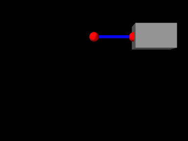
A simple rigid body-spring model is defined in
artisynth.demos.tutorial.RigidBodySpring
This differs from ParticleSpring only in the build() method, which is listed below:
The differences from ParticleSpring begin
at line 9. Instead of creating a second particle, a rigid body is
created using the factory method
RigidBody.createBox(), which
takes x, y, z widths and a (uniform) density and creates a box-shaped
rigid body complete with surface mesh and appropriate mass and
inertia. As the box is initially centered at the origin, moving it
elsewhere requires setting the body’s pose, which is done using setPose(). The RigidTransform3d passed to setPose() is
created using a three-argument constructor that generates a
translation-only transform. Next, starting at line 14, a FrameMarker is created for a location ![]() relative to the
rigid body, and attached to the body using its setFrame()
method.
relative to the
rigid body, and attached to the body using its setFrame()
method.
The remainder of build() is the same as for ParticleSpring, except that the spring is attached to the frame marker instead of a second particle.
3.2.3 Creating rigid bodies
As illustrated above, rigid bodies can be created using factory methods supplied by RigidBody. Some of these include:
The bodies do not need to be named; if no name is desired, then name can be specified as null.
In addition, there are also factory methods for creating a rigid body directly from a mesh:
These take either a polygonal mesh (Section 2.5), or a file name from which a mesh is read, and use it as the body’s surface mesh and then compute the mass and inertia properties from the specified (uniform) density.
When a body is created directly from a surface mesh, its center of mass will typically not be coincident with the origin of its coordinate frame. Section 3.2.6 discusses the implications of this and how to correct it.
Alternatively, one can create a rigid body directly from a constructor, and then set the mesh and inertia properties explicitly:
3.2.4 Pose and velocity
A body’s pose can be set and queried using the methods
These use a RigidTransform3d (Section
2.2) to describe the pose. Body poses are
described in world coordinates and specify the transform from body to
world coordinates. In particular, the pose for a body A specifies
the rigid transform ![]() .
.
Rigid bodies also expose the translational and rotational components of their pose via the properties position and orientation, which can be queried and set independently using the methods
The velocity of a rigid body is described using a Twist (Section 2.4), which contains both the translational and rotational velocities. The following methods set and query the spatial velocity as described with respect to world coordinates:
During simulation, unless a rigid body has been set to be parametric (Section 1.2.4), its pose and velocity are updated in response to forces, so setting the pose or velocity generally makes sense only for setting initial conditions. On the other hand, if a rigid body is parametric, then it is possible to control its pose during the simulation, but in that case it is better to set its target pose and/or target velocity, as described in Section 5.3.1.
3.2.5 Inertia and the surface mesh
The “mass” of a rigid body is described by its spatial inertia,
which is a ![]() matrix relating its spatial velocity to its
spatial momentum (Section A.6). Within
ArtiSynth, spatial inertia is described by a
SpatialInertia object, which
specifies its mass, center of mass (with respect to body coordinates),
and rotational inertia (with respect to the center of mass).
matrix relating its spatial velocity to its
spatial momentum (Section A.6). Within
ArtiSynth, spatial inertia is described by a
SpatialInertia object, which
specifies its mass, center of mass (with respect to body coordinates),
and rotational inertia (with respect to the center of mass).
Most rigid bodies are also associated with a polygonal surface mesh, which can be set and queried using the methods
The second method takes an optional fileName argument that can be set to the name of a file from which the mesh was read. Then if the model itself is saved to a file, the model file will specify the mesh using the file name instead of explicit vertex and face information, which can reduce the model file size considerably.
Rigid bodies can also have more than one mesh, as described in Section 3.2.9.
The inertia of a rigid body can be explicitly set using a variety of methods including
and can be queried using
In practice, it is often more convenient to simply specify a mass or a density, and then use the geometry of the surface mesh (and possibly other meshes, Section 3.2.9) to compute the remaining inertial values. How a rigid body’s inertia is computed is determined by its inertiaMethod property, which can be one of:
- EXPLICIT
-
Inertia is set explicitly.
- MASS
-
Inertia is determined implicitly from the mesh geometry and the body’s mass.
- DENSITY
-
Inertia is determined implicitly from the mesh geometry and the body’s density (which is multiplied by the mesh volume(s) to determine a mass).
When using DENSITY to determine the inertia, it is generally assumed that the contributing meshes are both polygonal and closed. Meshes which are either open or non-polygonal generally do not have a well-defined volume which can be multiplied by the density to determine the mass.
The inertiaMethod property can be set and queried using
and its default value is DENSITY. Explicitly setting the inertia using one of the setInertia() methods described above will set inertiaMethod to EXPLICIT. The method
will (re)compute the inertia using the mesh geometry and a density value and set inertiaMethod to DENSITY, and the method
will (re)compute the inertia using the mesh geometry and a mass value and set inertiaMethod to MASS.
Finally, the (assumed uniform) density of the body can be queried using
There are some subtleties involved in determining the inertia using either the DENSITY or MASS methods when the rigid body contains more than one mesh. Details are given in Section 3.2.9.
3.2.6 Coordinate frames and the center of mass
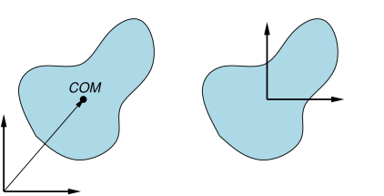
It is important to note that the origin of a body’s coordinate frame will not necessarily coincide with its center of mass (COM), and in fact the frame origin does not even have to lie inside the body’s surface (Figure 3.4). This typically occurs when a body’s inertia is computed directly from its surface mesh (or meshes), as described in Section 3.2.5.
Having the COM differ from the frame origin may lead to some undesired
effects. For instance, since the body’s spatial velocity is defined
with respect to the frame origin and not the COM, if the two are not
coincident, then a purely angular body velocity will cause the COM to
translate. The body’s spatial inertia also becomes more complicated,
with non-zero ![]() blocks in the lower left and upper right
(Section A.6), which can have a small effect on
computational accuracy. Finally, manipulating a body’s pose in the
ArtiSynth UI (as described in the section “Model Manipulation” in
the
ArtiSynth User Interface Guide) can
also be more cumbersome if the origin is located far from the COM.
blocks in the lower left and upper right
(Section A.6), which can have a small effect on
computational accuracy. Finally, manipulating a body’s pose in the
ArtiSynth UI (as described in the section “Model Manipulation” in
the
ArtiSynth User Interface Guide) can
also be more cumbersome if the origin is located far from the COM.
There are several ways to ensure that the COM and frame origin are coincident. The most direct is to call the method centerPoseOnCenterOfMass() after the body has been created:
This will shift the body’s frame to be coincident with the COM, while at the same time translating its mesh vertices in the opposite direction so that its mesh (or meshes) don’t move with respect to world coordinates. The spatial inertia is updated as well.
Alternatively, if the body is being created from a single mesh, one may transform that mesh to be centered on its COM before it is used to define the body. This can be done using the PolygonalMesh method translateToCenterOfVolume(), which centers a mesh’s vertices on its COM (assuming a uniform density):
3.2.7 Damping parameters
As with particles, it is possible to set damping parameters for rigid bodies. Damping can be specified in two different ways:
-
1.
Translational/rotational damping which is proportional to a body’s translational and rotational velocity;
-
2.
Inertial damping, which is proportional to a body’s spatial inertia multiplied by its spatial velocity.
Translational/rotational damping is controlled by the MechModel properties frameDamping and rotaryDamping, and generates a spatial force centered on each rigid body’s coordinate frame given by
| (3.0) |
where ![]() and
and ![]() are the frameDamping and rotaryDamping values, and
are the frameDamping and rotaryDamping values, and ![]() and
and ![]() are the translational
and angular velocity of the body’s coordinate frame. The damping
parameters can be set and queried using the MechModel methods
are the translational
and angular velocity of the body’s coordinate frame. The damping
parameters can be set and queried using the MechModel methods
These damping parameters can also be set for individual bodies using their own (inherited) frameDamping and rotaryDamping properties.
For models involving rigid bodies, it is often necessary to set rotaryDamping to a non-zero value because frameDamping will provide no damping at all when a rigid body is simply rotating about its coordinate frame origin.
Inertial damping is controlled by the MechModel property inertialDamping, and generates a spatial force centered on a rigid body’s coordinate frame given by
| (3.1) |
where ![]() is the inertialDamping,
is the inertialDamping, ![]() is the body’s
is the body’s ![]() spatial inertia matrix (Section A.6), and
spatial inertia matrix (Section A.6), and
![]() is the body’s spatial velocity. The inertial damping property
can be set and queried using the MechModel methods
is the body’s spatial velocity. The inertial damping property
can be set and queried using the MechModel methods
This parameter can also be set for individual bodies using their own (inherited) inertialDamping property.
Inertial damping offers two advantages over translational/rotational damping:
- 1.
It is independent of the location of the body’s coordinate frame with respect to its center of mass;
- 2.
There is no need to adjust two different translational and rotational parameters or to consider their relative sizes, as these considerations are contained within the spatial inertia itself.
3.2.8 Rendering rigid bodies
A rigid body is rendered in ArtiSynth by drawing its mesh (or meshes, Section 3.2.9) and/or coordinate frame.
Meshes are drawn using the face rendering properties described in more detail in Section 4.3. The most commonly used of these are:
-
•
faceColor: A value of type java.awt.Color giving the color of mesh faces. The default value is GRAY.
-
•
shading: A value of type Renderer.Shading indicating how the mesh should be shaded, with the options being FLAT, SMOOTH, METAL, and NONE. The default value is FLAT.
-
•
alpha: A double value between 0 and 1 indicating transparency, with transparency increasing as value decreases from 1. The default value is 1.
-
•
faceStyle: A value of type Renderer.FaceStyle indicating which face sides should be drawn, with the options being FRONT, BACK, FRONT_AND_BACK, and NONE. The default value is FRONT.
-
•
drawEdges: A boolean indicating whether the mesh edges should also be drawn, using either the edgeColor rendering property, or the lineColor property if edgeColor is not set. The default value is false.
-
•
edgeWidth: An integer giving the width of the mesh edges in pixels.
These properties, and others, can be set either interactively in the GUI, or in code. To set the render properties in the GUI, select the rigid body or its mesh component, and then right click the mouse and choose Edit render props .... More details are given in the section “Render properties” in the ArtiSynth User Interface Guide.
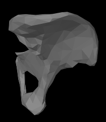 |
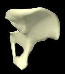 |
 |
Properties can also be set in code, usually during the build() method. Typically this is done using a static method of the RenderProps class that has the form
where XXX is the property name, comp is the component for which the property should be set, and value is the desired value. Some examples are shown in Figure 3.5 for a rigid body hip representation with a fairly coarse mesh. The left image shows the default rendering, using a gray color and flat shading. The center image shows a lighter color and smooth shading, which could be set by the following code fragment:
Finally, the right image shows the body rendered as a wire frame, which can be done by setting faceStyle to NONE and drawEdges to true:
Render properties can also be set in higher level model components, from which their values will be inherited by lower level components that have not explicitly set their own values. For example, setting the faceColor render property in the MechModel will automatically set the face color for all subcomponents which have not explicitly set faceColor. More details on render properties are given in Section 4.3.
 |
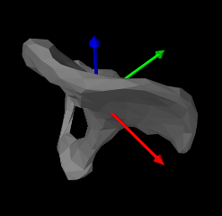 |
In addition to mesh rendering, it is often useful to draw a rigid
body’s coordinate frame, which can be done using its axisLength
and axisDrawStyle properties. Setting axisLength to a
positive value will cause the body’s three coordinate axes to be
drawn, with the indicated length, with the ![]() ,
, ![]() and
and ![]() axes
colored red, green, and blue, respectively. The axisDrawStyle
property controls how the axes are rendered (Figure
3.6). It has the type
Renderer.AxisDrawStyle, and can
be set to the following values:
axes
colored red, green, and blue, respectively. The axisDrawStyle
property controls how the axes are rendered (Figure
3.6). It has the type
Renderer.AxisDrawStyle, and can
be set to the following values:
- OFF
-
Axes are not rendered.
- LINE
-
Axes are rendered as simple red-green-blue lines, with a width given by the joint’s lineWidth rendering property.
- ARROW
-
Axes are rendered as solid red-green-blue arrows.
As with the rendering properties, the axisLength and axisDrawStyle properties can be managed either interactively in the GUI (by selecting the body, right clicking and choosing Edit properties ...), or in code, using the following methods:
3.2.9 Multiple meshes
A RigidBody may contain multiple meshes, which can be useful for various reasons:
-
•
It may be desirable to use different meshes for collision detection, inertia computation, and visual presentation;
-
•
Different render properties can be set for different mesh components, allowing the body to be rendered in a more versatile way;
-
•
Different mesh components can be selected individually.
Each rigid body mesh is encapsulated inside a RigidMeshComp component, which is in turn stored in a subcomponent list called meshes. Meshes do not need to be instances of PolygonalMesh; instead, they can be any instance of MeshBase, including PointMesh and PolylineMesh.
The default surface mesh, returned by getSurfaceMesh(), is also stored inside a RigidMeshComp in the meshes list. By default, the surface mesh is the first mesh in the list, but is otherwise defined to be the first mesh in meshes which is also an instance of PolygonalMesh. The RigidMeshComp containing the surface mesh can be obtained using the method getSurfaceMeshComp().
A RigidMeshComp contains a number of properties that control how the mesh is displayed and interacts with its rigid body:
- renderProps
-
Render properties controlling how the mesh is rendered (see Section 4.3).
- hasMass
-
A boolean, which if true means that the mesh will contribute to the body’s inertia when the inertiaMethod is either MASS or DENSITY. The default value is true.
- massDistribution
-
An enumerated type defined by MassDistribution which specifies how the mesh’s inertia contribution is determined for a given mass. VOLUME, AREA, LENGTH, and POINT indicate, respectively, that the mass is distributed evenly over the mesh’s volume, area (faces), length (edges), or points. The default value is determined by the mesh type: VOLUME for a closed PolygonalMesh, AREA for an open PolygonalMesh, LENGTH for a PolylineMesh, and POINT for a PointMesh. Applications can specify an alternate value providing the mesh has the features to support it. Specifying DEFAULT will restore the default value.
- isCollidable
-
- volume
-
A double whose value is the volume of the mesh. If the mesh is a PolygonalMesh, this is the value returned by its computeVolume() method. Otherwise, the volume is 0, unless setVolume(vol) is used to explicitly set a non-zero volume value.
- mass
-
A double whose default value is the product of the density and volume properties. Otherwise, if mass has been explicitly set using setMass(mass), the value is the explicit mass.
- density
-
A double whose default value is the rigid body’s density. Otherwise, if density has been explicitly set using setDensity(density), the value is the explicit density, or if mass has been explicitly set using setMass(mass), the value is the explicit mass divided by volume.
Note that by default, the density of a RigidMeshComp is simply the density setting for the rigid body, and the mass is this times the volume. However, it is possible to set either an explicit mass or a density value that will override this. (Also, explicitly setting a mass will unset any explicit density, and explicitly setting the density will unset any explicit mass.)
When the inertiaMethod of the rigid body is either MASS or
DENSITY, then its inertia is computed from the sum of all the
inertias ![]() of the component meshes
of the component meshes ![]() for which hasMass is
true. Each
for which hasMass is
true. Each ![]() is computed by the mesh’s
createInertia(mass,massDistribution) method,
using the mass and massDistribution properties of
its RigidMeshComp.
is computed by the mesh’s
createInertia(mass,massDistribution) method,
using the mass and massDistribution properties of
its RigidMeshComp.
When forming the body inertia from the inertia components of individual meshes, no attempt is made to account for mesh overlap. If this is important, the meshes themselves should be modified in advance so that they do not overlap, perhaps by using the CSG primitives described in Section 2.5.7.
Instances of RigidMeshComp can be created directly, using constructions such as
or
after which they can be added or removed from the meshes list using the methods
It is also possible to add meshes directly to the meshes list, using the methods
each of which creates a RigidMeshComp, adds it to the mesh list, and returns it. The second method also specifies the values of the hasMass and collidable properties (both of which are true by default).
3.2.10 Example: a composite rigid body
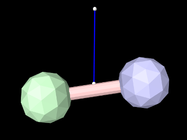
An example of constructing a rigid body from multiple meshes is defined in
artisynth.demos.tutorial.RigidCompositeBody
This uses three meshes to construct a rigid body whose shape resembles a dumbbell. The code, with the include files omitted, is listed below:
As in the previous examples, the build() method starts by creating a MechModel (lines 6-7). Three different meshes (two balls and an axis) are then constructed at lines 10-15, using MeshFactory methods (Section 2.5) and transforming each result to an appropriate position/orientation with respect to the body’s coordinate frame.
The body itself is constructed at lines 18-24. Its default density is set to 10, and its frame damping (Section 3.2.7) is also set to 10 (the previous rigid body example in Section 3.2.2 relied on spring damping to dissipate energy). The meshes are added using addMesh(), which allocates and returns a RigidMeshComp. For the ball meshes, these are saved in bcomp1 and bcomp2 and used later to adjust density and/or render properties.
Lines 27-34 create a simple linear spring, connected to a fixed point p0 and a marker mkr. The marker is created and attached to the body by the MechModel method addFrameMarkerWorld(), which places the marker at a known position in world coordinates. The spring is created using an AxialSpring constructor that accepts a name, along with stiffness, damping, and rest length parameters to specify a LinearAxialMaterial.
At line 37, bcomp1 is used to set the density of ball1 to 8. Since this is less than the default body density, the inertia component of ball1 will be lighter than that of ball2. Finally, render properties are set at lines 41-45. This includes setting the default face colors for the body and for each ball.
To run this example in ArtiSynth, select All demos > tutorial > RigidCompositeBody from the Models menu. The model should load and initially appear as in Figure 3.7. Running the model (Section 1.5.3) will cause the rigid body to fall and swing about under gravity, with the right ball (ball1) not falling as far because it has less density.
3.3 Mesh components
ArtiSynth models frequently incorporate 3D mesh geometry, as defined by the geometry classes PolygonalMesh, PolylineMesh, and PointMesh described in Section 2.5. Within a model, these basic classes are typically enclosed within container components that are subclasses of MeshComponent. Commonly used instances of these include
- RigidMeshComp
-
Introduced in Section 3.2.9, these contain the mesh geometry for rigid bodies, and are stored in a rigid body subcomponent list named meshes. Their mesh vertex positions are fixed with respect to their body’s coordinate frame.
- FemMeshComp
-
Contain mesh geometry associated with finite element models (Chapter 6), including surfaces meshes and embedded mesh geometry, and are stored in a subcomponent list of the FEM model named meshes. Their mesh vertex positions change as the FEM model deforms.
- SkinMeshBody
-
Described in detail in Chapter 11, these describe “skin” geometry that encloses both rigid bodies and/or FEM models. Their mesh vertex positions change as the underlying bodies move and deform. Skinning meshes may be placed anywhere, but are typically stored in the meshBodies component list of a MechModel.
- FixedMeshBody
-
Described further below, these store arbitrary mesh geometry (polygonal, polyline, and point) and provide (like rigid bodies) a rigid coordinate frame that allows the mesh to be positioned and oriented arbitrarily. As their name suggests, their mesh vertex positions are fixed with respect to this coordinate frame. Fixed body meshes may be placed anywhere, but are typically stored in the meshBodies component list of a MechModel.
3.3.1 Fixed mesh bodies
As mentioned above, FixedMeshBody can be used for placing arbitrary mesh geometry within an ArtiSynth model. These mesh bodies are non-dynamic: they do not interact or collide with other model components, and they function primarily as 3D graphical objects. They can be created from primary mesh components using constructors such as:
| FixedMeshBody (MeshBase mesh) |
Create an unnamed body containing a specified mesh. |
| FixedMeshBody (String name, MeshBase mesh) |
Create a named body containing a specified mesh. |
It should be noted that the primary meshes are not copied and are instead stored by reference, and so any subsequent changes to them will be reflected in the mesh body. As with rigid bodies, fixed mesh bodies contain a coordinate frame, or pose, that describes the position and orientation of the body with respect to world coordinates. Methods to control the pose include:
| RigidTransform3d getPose() |
Returns the pose of the body (with respect to world). |
| void setPose (RigidTransform3d XFrameToWorld) |
Sets the pose of the body. |
| Point3d getPosition() |
Returns the body position (pose translation component). |
| void setPosition (Point3d pos) |
Sets the body position. |
| AxisAngle getOrientation() |
Returns the body orientation (pose rotation component). |
| void setOrientation (AxisAngle axisAng) |
Sets the body orientation. |
Once created, a canonical place for storing mesh bodies is the MechModel component list meshBodies. Methods for maintaining this list include:
| ComponentListView<MeshComponent> meshBodies() |
Returns the meshBodies list. |
| void addMeshBody (MeshComponent mcomp) |
Adds mcomp to meshBodies. |
| boolean removeMeshBody (MeshComponent mcomp) |
Removes mcomp from meshBodies. |
| void clearMeshBodies() |
Clears the meshBodies list. |
Meshes used for instantiating fixed mesh bodies are typically read from files (Section 2.5.5), but can also be created using factory methods (Section 2.5.1). As an example, the following code fragment creates a torus mesh using a factory method, set its pose, and then adds it to a MechModel:
Rendering of mesh bodies is controlled using the same properties described in Section 3.2.8 for rigid bodies, including the renderProps subproperties faceColor, shading, alpha, faceStyle, and drawEdges, and the properties axisLength and axisDrawStyle for displaying a body’s coordinate frame.
3.3.2 Example: adding mesh bodies to MechModel
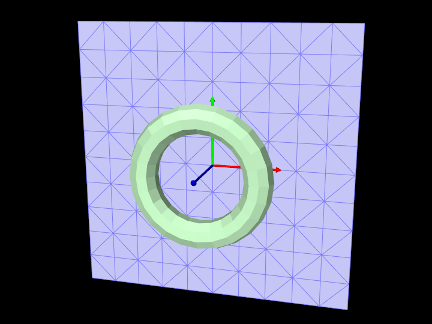
A simple application that creates a pair of fixed meshes and adds them to a MechModel is defined in
artisynth.demos.tutorial.FixedMeshes
The build() method for this is shown below:
After creating a MechModel (lines 3-4), a torus shaped mesh is imported from the file data/torus_9_24.obj (lines 8-16). As described in Section 2.6, the RootModel method getSourceRelativePath() is used to locate this file relative to the model’s source folder. The file path is used in the PolygonalMesh constructor, which is enclosed within a try/catch block to handle possible I/O exceptions. Once imported, the mesh is used to instantiate a FixedMeshBody named "torus" which is added to the MechModel (lines 18-19).
Another mesh, representing a square, is created with a factory method
and used to instantiate a mesh body named "square" (lines
22-26). The factory method specifies both the size and triangle
density of the mesh in the ![]() -
-![]() plane. Once created, the square’s
pose is set to a 90 degree rotation about the
plane. Once created, the square’s
pose is set to a 90 degree rotation about the ![]() axis and a
translation of 0.5 along
axis and a
translation of 0.5 along ![]() (lines 28-29).
(lines 28-29).
Rendering properties are set at lines 33-41. The torus is made pale green by setting its face color; the coordinate frame for the square is made visible as solid arrows using the axisLength and axisDrawStyle properties; and the square is made blue gray, with its edges made visible and drawn using a darker color, and its face style set to FRONT_AND_BACK so that it’s visible from either side.
To run this example in ArtiSynth, select All demos > tutorial > FixedMeshes from the Models menu. The model should load and initially appear as in Figure 3.8.
3.4 Joints and connectors
In a typical mechanical model, many of the rigid bodies are interconnected, either using spring-type components that exert binding forces on the bodies, or through joints and connectors that enforce the connection using hard constraints. This section describes the latter. While the discussion focuses on rigid bodies, joints and connectors can be used more generally with any body that implements the ConnectableBody interface. In particular, this allows joints to also interconnect finite element models, as described in Section 6.6.4.
3.4.1 Joints and coordinate frames
Consider two rigid bodies A and B. The pose of body B with respect to
body A can be described by the 6 DOF rigid transform ![]() . If A
and B are unconnected,
. If A
and B are unconnected, ![]() may assume any possible value and has
a full six degrees of freedom. A joint between A and B
constrains the set of poses that are possible between the two bodies
and reduces the degrees of freedom available to
may assume any possible value and has
a full six degrees of freedom. A joint between A and B
constrains the set of poses that are possible between the two bodies
and reduces the degrees of freedom available to ![]() . For ease
of use, the constraining action of a joint is described with respect
to a pair of local coordinate frames C and D that are connected to
frames A and B, respectively, by auxiliary transformations. This
allows joints to be placed at locations that do not correspond
directly to frames A or B.
. For ease
of use, the constraining action of a joint is described with respect
to a pair of local coordinate frames C and D that are connected to
frames A and B, respectively, by auxiliary transformations. This
allows joints to be placed at locations that do not correspond
directly to frames A or B.
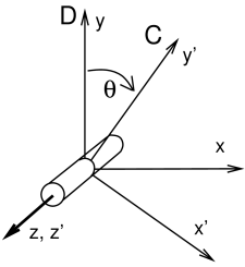
The joint frames C and D move with respect to each other as the joint
moves. The allowed joint motions therefore correspond to the allowed
values of the joint transform ![]() . Although both frames
typically move with their attached bodies, D is considered the base frame and C the motion frame (this is because when a joint
is used to connect a single body to ground, body B is set to null and the world frame takes its place). As an example of a
joint’s constraining effect, consider a hinge joint (Figure
3.9), which allows C to move with respect to D only by
rotating about the
. Although both frames
typically move with their attached bodies, D is considered the base frame and C the motion frame (this is because when a joint
is used to connect a single body to ground, body B is set to null and the world frame takes its place). As an example of a
joint’s constraining effect, consider a hinge joint (Figure
3.9), which allows C to move with respect to D only by
rotating about the ![]() axis while the origins of C and D remain
coincident. Other motions are prohibited. If we let
axis while the origins of C and D remain
coincident. Other motions are prohibited. If we let ![]() describe
the counter-clockwise rotation angle of C about the
describe
the counter-clockwise rotation angle of C about the ![]() axis, then
axis, then
![]() should always have the form
should always have the form
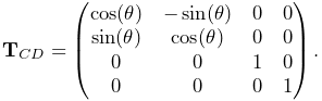 |
(3.1) |
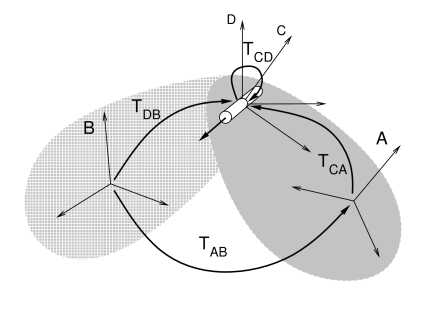
When a joint is attached to bodies A and B, frame C is fixed to body A
and frame D is fixed to body B. Except in special cases, the joint
frames C and D are not coincident with the body frames A
and B. Instead, they are located relative to A and B by the
transforms ![]() and
and ![]() , respectively
(Figure 3.10). Since
, respectively
(Figure 3.10). Since ![]() and
and ![]() are
both fixed, the joint constraints on
are
both fixed, the joint constraints on ![]() constrain the relative
poses of A and B, with
constrain the relative
poses of A and B, with ![]() determined from
determined from
| (3.2) |
(See Section A.2 for a discussion of determining transforms between related coordinate frames).
3.4.2 Joint coordinates, constraints, and errors
Each different joint and connector type restricts the motion between
two bodies to ![]() degrees of freedom, for some
degrees of freedom, for some ![]() . Sometimes,
the joint also defines a set of
. Sometimes,
the joint also defines a set of ![]() coordinates that parameterize
these
coordinates that parameterize
these ![]() DOFs. For example, the hinge joint described above is
parameterized by
DOFs. For example, the hinge joint described above is
parameterized by ![]() . Other examples are given in
Section 3.5: a 2 DOF cylindrical has coordinates
. Other examples are given in
Section 3.5: a 2 DOF cylindrical has coordinates ![]() and
and ![]() , a 3 DOF gimbal joint is parameterized by the
roll-pitch-yaw angles
, a 3 DOF gimbal joint is parameterized by the
roll-pitch-yaw angles ![]() ,
, ![]() , and
, and ![]() , etc. When
, etc. When
![]() (where
(where ![]() is the identity transform), the coordinates
are usually all equal to zero, and the joint is said to be in the zero state.
is the identity transform), the coordinates
are usually all equal to zero, and the joint is said to be in the zero state.
As explained in Section 1.2.3, ArtiSynth uses a
full coordinate formulation for dynamic simulation. That means that
instead of using joint coordinates to describe system state, it uses
the combined full coordinates ![]() of all dynamic components. For
example, a model consisting of a single rigid body connected to ground
by a hinge joint will have 6 DOF (corresponding to the 6 DOF of the
body), rather than the 1 DOF implied by the hinge joint. The DOF
restrictions imposed by the joints are then enforced by a set of
linearized constraint relationships
of all dynamic components. For
example, a model consisting of a single rigid body connected to ground
by a hinge joint will have 6 DOF (corresponding to the 6 DOF of the
body), rather than the 1 DOF implied by the hinge joint. The DOF
restrictions imposed by the joints are then enforced by a set of
linearized constraint relationships
| (3.3) |
that restrict the body velocities ![]() computed at each simulation
step, usually by solving an MLCP like (1.13). As
explained in Section 1.2.3, the right side
vectors
computed at each simulation
step, usually by solving an MLCP like (1.13). As
explained in Section 1.2.3, the right side
vectors ![]() and
and ![]() in (3.3) contain time
derivative terms, which for simplicity much of the following
presentation will assume to be 0.
in (3.3) contain time
derivative terms, which for simplicity much of the following
presentation will assume to be 0.
Each joint contributes its own set of constraint equations to (3.3). Typically these take the form of bilateral, or equality, constraints
| (3.4) |
which are added to the system’s global bilateral constraint matrix
![]() .
. ![]() contains
contains ![]() rows providing
rows providing ![]() individual
constraints
individual
constraints ![]() .
During simulation, these give rise to
.
During simulation, these give rise to ![]() constraint
forces (corresponding to
constraint
forces (corresponding to ![]() in (1.10))
which enforce the constraints.
in (1.10))
which enforce the constraints.
In some cases, the joint also maintains unilateral, or inequality
constraints, to keep ![]() out of inadmissible regions. These take
the form
out of inadmissible regions. These take
the form
| (3.5) |
and are added to the system’s global unilateral constraint matrix
![]() . They give rise to constraint forces corresponding to
. They give rise to constraint forces corresponding to ![]() in
(1.10). A common use of unilateral constraints
is to enforce range limits of the joint coordinates (Section
3.4.5), such as
in
(1.10). A common use of unilateral constraints
is to enforce range limits of the joint coordinates (Section
3.4.5), such as
| (3.6) |
A specific unilateral constraint is added to ![]() only when
only when
![]() is on or within the boundary of the inadmissible region
associated with that constraint. The constraint is then said to be
engaged. The combined number of bilateral and engaged unilateral
constraints for a particular joint should not exceed 6; otherwise, the
joint would be overconstrained.
is on or within the boundary of the inadmissible region
associated with that constraint. The constraint is then said to be
engaged. The combined number of bilateral and engaged unilateral
constraints for a particular joint should not exceed 6; otherwise, the
joint would be overconstrained.
Joint coordinates, when supported for a particular joint, can be both
read and set. Setting a coordinate causes the joint transform
![]() to change. To accommodate this, the system adjusts the poses
of one or both bodies connected to the joint, along with adjacent
bodies connected to them, with preference given to bodies that are not
attached to “ground”. However, if this is done during simulation,
and particularly if one or both of the bodies connected to the joint
are moving dynamically, the results will be unpredictable and will
likely conflict with the simulation.
to change. To accommodate this, the system adjusts the poses
of one or both bodies connected to the joint, along with adjacent
bodies connected to them, with preference given to bodies that are not
attached to “ground”. However, if this is done during simulation,
and particularly if one or both of the bodies connected to the joint
are moving dynamically, the results will be unpredictable and will
likely conflict with the simulation.
Joint coordinates are also often exported as properties. For example,
the
HingeJoint
class (Section 3.5) exports its ![]() coordinate
as the property theta, which can be accessed in the GUI, or via
the accessor methods
coordinate
as the property theta, which can be accessed in the GUI, or via
the accessor methods
Since joint constraints are generally nonlinear, their linearized
enforcement at the velocity level by (3.3) will
usually produce small errors as the simulation proceeds. These errors
are reduced using a position correction step described in
Section 4.9.1 and [11].
Errors can also be caused by joint compliance
(Section 3.4.9). Both effects mean that the joint
transform ![]() may deviate from the allowed values dictated by
the joint type. In ArtiSynth, this is accounted for by introducing an
additional constraint frame G between D and C
(Figure 3.11). G is computed to be the nearest frame
to C that lies exactly in the joint constraint space.
may deviate from the allowed values dictated by
the joint type. In ArtiSynth, this is accounted for by introducing an
additional constraint frame G between D and C
(Figure 3.11). G is computed to be the nearest frame
to C that lies exactly in the joint constraint space. ![]() is
therefore a valid joint transform,
is
therefore a valid joint transform, ![]() accommodates the error,
and the whole joint transform is given by the composition
accommodates the error,
and the whole joint transform is given by the composition
| (3.7) |
If there is no compliance or joint error, then frames G and C are
identical, ![]() , and
, and ![]() . Because
. Because ![]() describes the joint error, we sometimes refer to it as
describes the joint error, we sometimes refer to it as ![]() .
.

3.4.3 Creating joints
Joint and connector components in ArtiSynth are both derived from the superclass BodyConnector, with joints being further derived from JointBase, which provides support for coordinates. Some of the commonly used joints and connectors are described in Section 3.5.
An application creates a joint by constructing it and adding it to a MechModel. For this, two things need to be specified:
-
1.
The bodies A and B being connected;
-
2.
The initial locations of the C and D frames.
For the second item, it is often more convenient to specify C and D in world
coordinates, i.e., as ![]() and
and ![]() , and then determine
, and then determine ![]() and
and
![]() from
from
| (3.8) | ||||
| (3.9) |
where ![]() and
and ![]() are the current poses of A and B.
are the current poses of A and B.
Many joints have constructors of the form
which specifies only ![]() and the bodies A and B. The constructor
then computes
and the bodies A and B. The constructor
then computes ![]() from
from
| (3.10) |
where ![]() is the joint’s initial
is the joint’s initial ![]() value returned by
getCurrentTCD(). For joints
with coordinates, the initial
value returned by
getCurrentTCD(). For joints
with coordinates, the initial ![]() is determined from the initial
coordinate values (which are usually 0). Typically (but not always), the
initial
is determined from the initial
coordinate values (which are usually 0). Typically (but not always), the
initial ![]() is also the identity, so that
is also the identity, so that ![]() .
.
After the joint is created, it should be added to the system’s MechModel using addBodyConnector(), as shown in the following code fragment:
Joints usually offer a number of other constructors that let its world location and body relationships to be specified in different ways. These may include:
The first, which is restricted to rigid bodies, allows the application
to explicitly specify transforms ![]() and
and ![]() connecting
frames C and D to the body frames A and B, and is useful when
connecting
frames C and D to the body frames A and B, and is useful when
![]() and
and ![]() are explicitly known, or the initial value of
are explicitly known, or the initial value of
![]() is not the identity. Likewise, the second constructor
allows
is not the identity. Likewise, the second constructor
allows ![]() and
and ![]() to be explicitly specified, with
to be explicitly specified, with
![]() if
if ![]() . For instance, suppose
. For instance, suppose
![]() and
and ![]() are both known. Then we can use the
relationship
are both known. Then we can use the
relationship
| (3.11) |
to create the joint as in the following code fragment:
As an alternative to specifying ![]() or its equivalents, some
joint types provide constructors that let the application locate
specific joint features. These may be easier to use in some cases. For
instance, HingeJoint provides a
constructor
or its equivalents, some
joint types provide constructors that let the application locate
specific joint features. These may be easier to use in some cases. For
instance, HingeJoint provides a
constructor
that specifies origin of D and its ![]() axis (which is the rotation
axis), with the remaining orientation of D aligned as closely as
possible with the world.
SphericalJoint provides a
constructor
axis (which is the rotation
axis), with the remaining orientation of D aligned as closely as
possible with the world.
SphericalJoint provides a
constructor
that specifies origin of D and aligns its orientation with the world. Users should consult the source code or API documentation for specific joints to see what special constructors may be available.
It is also possible to use a joint to connect a single body to “ground” (i.e., the world frame). When this is done, the body in question is always bodyA, and bodyB is null. Most joints provide a constructor of the form
which allows this to be done explicitly. Alternatively, most joint constructors which supply body B will allow this to be specified as null, so that body A will be connected to ground by default.
When using joints to build an articulated structure, the usual convention is for bodyA to be on the distal, or “outer”, side of the joint and for bodyB to be on the proximal, or “inner”, side.
Finally, it is also possible to create a joint using its default constructor and attach it to the bodies afterward, using the various setBodies() methods:
| void setBodies (ConnectableBody bodyA, ConnectableBody bodyB, RigidTransform3d TDW) |
Set A and B given TDW. |
| void setBodies (ConnectableBody bodyA, ConnectableBody bodyB, RigidTransform3d TCW, RigidTransform3d TDW) |
Set A and B given TCW and TDW. |
| void setBodies (RigidBody bodyA, RigidTransform3d TCA, RigidBody bodyB, RigidTransform3d TDB) |
Set A and B given TCA and TDB. |
| void setBodies (ConnectableBody bodyA, FrameAttachment attachmentA, ConnectableBody bodyB, FrameAttachment attachmentB) |
Set A and B with custom attachments. |
| void setBodyA (ConnectableBody bodyA, RigidTransform3d TCW) |
Set A given TCW. |
| void setBodyA (ConnectableBody bodyA, FrameAttachment attachmentA) |
Set A with custom attachment. |
| void setBodyB (ConnectableBody bodyB, RigidTransform3d TDW) |
Set B given TDW. |
| void setBodyB (ConnectableBody bodyB, FrameAttachment attachmentB) |
Set B with custom attachment. |
As with the constructors, TDW and TCW give the locations of D and C in world coordinates, and if TCW is needed but not specified, it is computed per equation (3.10). bodyB can also be given as null, which will cause body A to be attached to ground. The methods specifying FrameAttachments allow for situations where special attachment types are needed, such as when connecting joints to finite element models (Section 6.6.4). The setBodyA() and setBodyB() methods connect body A (or body B) while leaving body B (or body A) alone, and are useful when it is necessary to set (or reset) only one body connection.
The following example creates a HingeJoint using setBodies():
A more complicated, but exactly equivalent, version using setBodyA() and setBodyB() is given by
One reason for using setBodies() is that it allows the joint transform
![]() to be modified (by setting coordinate values) before setBodies() is called; this is discussed further in
Section 3.4.4.
to be modified (by setting coordinate values) before setBodies() is called; this is discussed further in
Section 3.4.4.
3.4.4 Working with coordinates
As mentioned in Section 3.4.2, some joints
support coordinates that parameterize the valid motions within the
joint transform ![]() . All such joints are subclasses of
JointBase,
which provides some generic methods for querying and setting
coordinate values (JointBase is in turn a subclass of
BodyConnector).
. All such joints are subclasses of
JointBase,
which provides some generic methods for querying and setting
coordinate values (JointBase is in turn a subclass of
BodyConnector).
The number of coordinates is returned by the method numCoordinates(); if this returns 0, then coordinates are not
supported. Each coordinate has an index in the range ![]() ,
where
,
where ![]() is the number of coordinates. Coordinate values can be
queried or set using the following methods:
is the number of coordinates. Coordinate values can be
queried or set using the following methods:
Specific joint types usually also provide names for their joint
coordinates, along with integer constants describing their indices
and methods for accessing their values. For example,
CylindricalJoint
supports two coordinates, ![]() and
and ![]() , along with
the following:
, along with
the following:
The coordinate values are also exported as the properties z and theta, allowing them to be set in the GUI. For convenience, particularly in GUI applications, the properties and methods for controlling specific angular coordinates generally use degrees instead of radians.
It is recommended to call setCoordinate methods only after a joint has been added to its MechModel, in order to ensure that other bodies in its articulated structure, together with any muscle wrap paths (Chapter 9), are updated appropriately.
As discussed in Section 3.4.2, unlike in some multibody simulation systems (such as OpenSim), joint coordinates are not fundamental quantities that describe system state. As such, then, coordinates can usually only be set in specific circumstances that avoid simulation conflicts. In general, when joint coordinates are set, the system adjusts the poses of one or both bodies connected to this joint, along with adjacent bodies connected to them, with preference given to bodies that are not attached to “ground”. However, if this is done during simulation, and particularly if one or both of the bodies connected to the joint are moving dynamically, the results will be unpredictable and will likely conflict with the simulation.
Coordinate setting is discussed in greater detail in Section 3.6, along with the CoordinateSetter class that can be used to set coordinate values across several joints simultaneously.
If a joint has been created with its default constructor and not yet
attached to any bodies, then setting joint values will simply set the
joint transform ![]() . This can be useful in situations where one
needs to initialize a joint’s
. This can be useful in situations where one
needs to initialize a joint’s ![]() to a non-identity value
corresponding to a particular set of joint coordinates:
to a non-identity value
corresponding to a particular set of joint coordinates:
This can also be done in vector form:
In either of these cases, setBodies() will not use ![]() but instead use the value determined by the initial coordinate
values.
but instead use the value determined by the initial coordinate
values.
To determine the ![]() corresponding to a particular set of
coordinates, one may use the method
corresponding to a particular set of
coordinates, one may use the method
In some cases, within a model’s build() method, one may wish to set initial coordinates after a joint has been attached to its bodies, in order to move those bodies (along with the bodies attached to them) into an initial configuration without having to explicitly calculate the poses from the joint coordinates. As mentioned above, the system will make a decision about which attached bodies are most “free” and adjust their poses accordingly. This is done in the example of the next section.
3.4.5 Coordinate limits and locking
It is possible to set limits on a joint coordinate’s range, and also to lock a coordinate in place at its current value.
When a joint coordinate hits either an upper or lower range limit, a unilateral constraint is invoked to prevent it from violating the limit, and remains engaged until the joint moves away from the limit. Each range constraint that is engaged reduces the number of joint DOFs by one.
By default, joint range limits are usually disabled (i.e., they are
set to ![]() ). They can be queried and set, for a given
joint with index idx, using the methods:
). They can be queried and set, for a given
joint with index idx, using the methods:
where range limits for angular coordinates are specified in radians. For convenience, the following methods are also provided which use degrees instead of radians for angular coordinates:
Range checking can be disabled by setting the range to
![]() , or by specifying rng as null, which
implicitly does the same thing.
, or by specifying rng as null, which
implicitly does the same thing.
Ranges for angular coordinates are not limited to
but can instead be set to larger values; the joint will continue to wrap until the limit is reached.
Joint coordinates can also be locked, so that they hold their current value and don’t move. A joint is locked using a bilateral constraint that prevents motion in either direction and reduces the joint’s DOF count by one. The following methods are available for querying or setting a coordinate’s locked status:
As with coordinate values, specific joint types usually provide methods for controlling the ranges and locking status of individual coordinates, with ranges for angular coordinates specified in degrees instead of radians. For example, CylindricalJoint supplies the methods
The range and locking information is also exported as the properties zRange, thetaRange, zLocked, and thetaLocked, allowing them to be set in the GUI.
3.4.6 Example: a simple hinge joint
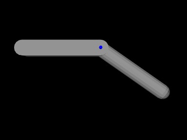
A simple model showing two rigid bodies connected by a joint is defined in
artisynth.demos.tutorial.RigidBodyJoint
The build method for this model is given below:
A MechModel is created as usual at line 4. However, in this
example, we also set some parameters for it:
setGravity() is
used to set the gravity acceleration vector to ![]() instead
of the default value of
instead
of the default value of ![]() , and the frameDamping
and rotaryDamping properties (Section
3.2.7) are set to provide appropriate damping.
, and the frameDamping
and rotaryDamping properties (Section
3.2.7) are set to provide appropriate damping.
Each of the two rigid bodies are created from a mesh and a density. The meshes themselves are created using the factory methods MeshFactory.createRoundedBox() and MeshFactory.createRoundedCylinder() (lines 13 and 22), and then RigidBody.createFromMesh() is used to turn these into rigid bodies with a density of 0.2 (lines 17 and 25). The pose of the two bodies is set using RigidTransform3d objects created with x, y, z translation and axis-angle orientation values (lines 18 and 26).
The hinge joint is implemented using HingeJoint, which is constructed at line 32 with the joint coordinate frame D being located in world coordinates by TDW as described in Section 3.4.3.
Once the joint is created and added to the MechModel, the method
setTheta() is
used to explicitly set the joint parameter to 35 degrees. The joint
transform ![]() is then set appropriately and bodyA is moved
to accommodate this (bodyA being chosen since it is the most
free to move).
is then set appropriately and bodyA is moved
to accommodate this (bodyA being chosen since it is the most
free to move).
Finally, joint rendering properties are set starting at line 42. We render the joint as a cylindrical shaft about the rotation axis, using its shaftLength and shaftRadius properties. Joint rendering is discussed in more detail in Section 3.4.11).
3.4.7 Joint coordinate handles
The class JointCoordinateHandle is a convenience class that encapsulates access to a single coordinate by containing both its joint and index within that joint. It can be easily constructed as follows,
and offers a number of methods to directly access coordinate properties:
| double getValue() |
Returns the value (in radians for rotary coordinates). |
| double getValueDeg() |
Returns the value (in degrees for rotary coordinates). |
| String getName() |
Queries the coordinate’s name. |
| JointBase getJoint() |
Returns the coordinate’s joint. |
| int getIndex() |
Queries the coordinate’s index within the joint. |
| MotionType getMotionType() |
Queries the coordinate’s motion type. |
| DoubleInterval getValueRange() |
Returns the range (in radians for rotary coordinates). |
| void setValueRange(DoubleInterval range) |
Sets the range (in radians for rotary coordinates). |
| DoubleInterval getValueRangeDeg() |
Returns the coordinate’s range (in degrees for rotary coordinates). |
| void setValueRangeDeg(DoubleInterval range) |
Sets the range (in degrees for rotary coordinates). |
| boolean isLocked() |
Queries whether the coordinate is locked. |
| void setLocked (boolean locked) |
Sets whether the coordinate is locked. |
3.4.8 Constraint forces
During each simulation solve step, the joint velocity constraints
described by (3.4) and (3.5) are
enforced by bilateral and unilateral constraint forces ![]() and
and
![]() :
:
| (3.11) |
Here, ![]() and
and ![]() are spatial forces (or wrenches, Section
A.5) acting in the joint coordinate
frame C, and
are spatial forces (or wrenches, Section
A.5) acting in the joint coordinate
frame C, and ![]() and
and ![]() are the Lagrange multipliers
computed as part of the mechanical system solve (see
(1.13) and (1.10)). The sizes
of
are the Lagrange multipliers
computed as part of the mechanical system solve (see
(1.13) and (1.10)). The sizes
of ![]() and
and ![]() equal the number of bilateral and engaged unilateral constraints in the joint; these numbers can be
queried for a particular joint using the methods
numBilateralConstraints()
and
numEngagedUnilateralConstraints().
(The number of engaged unilateral constraints may be less than the
total number of unilateral constraints; the latter may be queried with
numUnilateralConstraints(),
while the total number of
constraints is returned by
numConstraints().
equal the number of bilateral and engaged unilateral constraints in the joint; these numbers can be
queried for a particular joint using the methods
numBilateralConstraints()
and
numEngagedUnilateralConstraints().
(The number of engaged unilateral constraints may be less than the
total number of unilateral constraints; the latter may be queried with
numUnilateralConstraints(),
while the total number of
constraints is returned by
numConstraints().
Applications may sometimes need to query the current constraint force values, typically from within a controller or monitor (Section 5.3). The Lagrange multipliers themselves may be obtained with
which load the multipliers into lam or the and set their sizes to the number of bilateral or engaged unilateral constraints. Alternatively, one can retrieve the individual multiplier for the constraint indexed by idx using
Typically, it is more useful to find the spatial constraint forces
![]() and
and ![]() , which can be obtained with respect to frame C:
, which can be obtained with respect to frame C:
If the attached bodies A and B are rigid bodies, it is also possible to obtain the constraint wrenches experienced by those bodies:
Constraint wrenches obtained for bodies A or B are given in world
coordinates, which is consistent with the forces reported by rigid
bodies via their getForce() method. To orient the forces into
body coordinates, one may use the inverse of the rotation matrix ![]() of the body’s pose. For example:
of the body’s pose. For example:
3.4.9 Compliance and regularization
By default, the constraints used to implement joints and couplings are treated as hard, so that the system tries to respect the constraint conditions (3.3) as exactly as possible as the simulation proceeds. Sometimes, however, it is desirable to introduce some “softness” into the constraints, whereby constraint forces are determined as a linear function of their distance from the constraint. Adding compliance also allows an application to regularize a system of joint constraints that would otherwise be overconstrained, as illustrated in Section 3.4.10.
To describe compliance precisely, consider the bilateral constraint
portion of the MLCP in (1.13), which solves for the
updated system velocities ![]() at each time step:
at each time step:
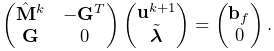 |
(3.12) |
Here ![]() is the system’s bilateral constraint matrix,
is the system’s bilateral constraint matrix, ![]() denotes
the constraint impulses (from which the constraint forces
denotes
the constraint impulses (from which the constraint forces ![]() can be
determined by
can be
determined by ![]() ), the regularization term
), the regularization term ![]() is zero,
and for simplicity we have assumed that
is zero,
and for simplicity we have assumed that ![]() is constant and so the
is constant and so the ![]() offset
on the lower right side is
offset
on the lower right side is ![]() .
.
Solving (3.12) results in constraint forces that satisfy
![]() precisely, corresponding to hard constraints. To
implement soft constraints, start by defining a function
precisely, corresponding to hard constraints. To
implement soft constraints, start by defining a function ![]() that defines the distances from each constraint, where
that defines the distances from each constraint, where ![]() is the
vector of system positions; these distances are
the local translational and rotational deviations from each
constraint’s correct position and are discussed in more detail in
Section 4.9.1. Then assume that the constraint
forces are a linear function of these distances:
is the
vector of system positions; these distances are
the local translational and rotational deviations from each
constraint’s correct position and are discussed in more detail in
Section 4.9.1. Then assume that the constraint
forces are a linear function of these distances:
| (3.13) |
where ![]() is a diagonal compliance matrix that is equivalent to
an inverse stiffness matrix. We also note that
is a diagonal compliance matrix that is equivalent to
an inverse stiffness matrix. We also note that ![]() will be time
varying, and that we can approximate its change between time steps as
will be time
varying, and that we can approximate its change between time steps as
| (3.14) |
Next, assume that in using (3.13) to determine ![]() for a particular time step, we use the average value of
for a particular time step, we use the average value of ![]() over the step, represented by
over the step, represented by ![]() .
Substituting this and (3.14) into
(3.13), multiplying by
.
Substituting this and (3.14) into
(3.13), multiplying by ![]() , and rearranging yields:
, and rearranging yields:
| (3.15) |
Then noting that ![]() , we obtain
a revised form of (3.12),
, we obtain
a revised form of (3.12),
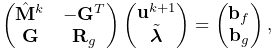 |
(3.16) |
in which ![]() and
and ![]() contain compliance terms defined by
contain compliance terms defined by
The resulting constraint behavior is different from that of (3.12) in two important ways:
-
1.
The joint now allows 6 DOF, with motion along the constrained directions limited by restoring spring constants given by the reciprocals of the diagonal entries of
 .
. - 2.
Unilateral constraints can be regularized using the same approach,
with a distance function defined such that ![]() .
.
The reason for specifying soft constraints using compliance instead of
stiffness is that by setting ![]() we can easily handle the case of
infinite stiffness where the constraints are strictly enforced.
The ArtiSynth compliance implementation uses a slightly more complex
version of (3.16) that accounts for non-constant
we can easily handle the case of
infinite stiffness where the constraints are strictly enforced.
The ArtiSynth compliance implementation uses a slightly more complex
version of (3.16) that accounts for non-constant ![]() and
also allows for a damping term
and
also allows for a damping term ![]() , where
, where ![]() is again a
diagonal matrix. For more details, see [9]
and [21].
is again a
diagonal matrix. For more details, see [9]
and [21].
When using compliance, damping is often needed for stability, and, in the case of unilateral constraints, to prevent “bouncing”. A good choice for damping is usually critical damping, which is discussed further below.
Any joint which is a subclass of
BodyConnector allows
individual compliance values ![]() and damping values
and damping values ![]() to be set
for each of the joint’s
to be set
for each of the joint’s ![]() constraints. These values comprise the
diagonal entries in the compliance and damping matrices
constraints. These values comprise the
diagonal entries in the compliance and damping matrices ![]() and
and ![]() ,
and can be queried and set using the methods
,
and can be queried and set using the methods
The vectors supplied to the above set methods contain the
requested compliance or damping values. If their size ![]() is less than
numConstraints(), then compliance or damping will be set for the
first
is less than
numConstraints(), then compliance or damping will be set for the
first ![]() constraints. Damping for a specific constraint only has an
effect if the compliance for that constraint is nonzero.
constraints. Damping for a specific constraint only has an
effect if the compliance for that constraint is nonzero.
What compliance and damping values should be specified? Compliance is
usually relatively easy to figure out. Each of the joint’s individual
constraints ![]() corresponds to a row in its bilateral constraint matrix
corresponds to a row in its bilateral constraint matrix
![]() or unilateral constraint matrix
or unilateral constraint matrix ![]() , and represents a
specific 6 DOF direction along which the spatial velocity
, and represents a
specific 6 DOF direction along which the spatial velocity
![]() (of frame C with respect to D) is restricted (more
details on this are given in Section 4.9.1).
Each of these constraint directions is usually predominantly linear or
rotational; specific descriptions for the constraints of different
joints are provided in Section 3.5. To determine
compliance for a constraint
(of frame C with respect to D) is restricted (more
details on this are given in Section 4.9.1).
Each of these constraint directions is usually predominantly linear or
rotational; specific descriptions for the constraints of different
joints are provided in Section 3.5. To determine
compliance for a constraint ![]() , estimate the typical force
, estimate the typical force ![]() likely
to act along its direction, decide how much displacement
likely
to act along its direction, decide how much displacement ![]() (translational or rotational) along that constraint is desirable, and
then set the compliance
(translational or rotational) along that constraint is desirable, and
then set the compliance ![]() to the associated inverse stiffness:
to the associated inverse stiffness:
| (3.17) |
Once ![]() is determined, the damping
is determined, the damping ![]() can be estimated based on
the desired damping ratio
can be estimated based on
the desired damping ratio ![]() , using the formula
, using the formula
| (3.18) |
where ![]() is the total mass of the bodies attached to the joint.
Typically, the desired damping will be close to critical damping, for
which
is the total mass of the bodies attached to the joint.
Typically, the desired damping will be close to critical damping, for
which ![]() .
.
Constraints associated with linear motion will typically require different compliance values from those associated with rotation. To make this process easier, joint components allow the setting of collective compliance values for their linear and rotary constraints, using the methods
The set() methods will set a uniform compliance for all linear or rotary constraints, except for unilateral constraints associated with coordinate limits. At the same time, they will also set an automatically computed critical damping value. Likewise, the get() methods query these linear or rotary constraints for uniform compliance values (with the corresponding critical damping), and return either that value, or -1 if it does not exist.
Most of the demonstration models for the joints described in Section 3.5 allow these linear and rotary compliance settings to be adjusted interactively using a control panel, enabling users to experimentally gain a feel for their behavior.
To determine programmatically whether a particular constraint is linear or rotary, one can use the joint method
which returns a vector of information flags for all its constraints. Linear and rotary constraints are indicated by the flags LINEAR and ROTARY, defined in RigidBodyConstraint.
3.4.10 Example: an overconstrained linkage
Situations may occasionally arise in which a model is overconstrained, which means that the rows of the bilateral
constraint matrix ![]() in (3.3) are not all
linearly dependent, or in other words,
in (3.3) are not all
linearly dependent, or in other words, ![]() does not have full
row rank. At present, the ArtiSynth solver has difficultly handling
overconstrained models, but these situations can often be handled by
adding a small amount of compliance to the
constraints. (Overconstraining is not a problem with unilateral
constraints
does not have full
row rank. At present, the ArtiSynth solver has difficultly handling
overconstrained models, but these situations can often be handled by
adding a small amount of compliance to the
constraints. (Overconstraining is not a problem with unilateral
constraints ![]() , because of the way they are handled by the solver.)
, because of the way they are handled by the solver.)
One possible symptom of an overconstrained system is an error message in the application’s terminal output, such as
Pardiso: num perturbed pivots=12
Overconstraining frequently occurs in closed-chain linkages, involving loops in which a jointed sequence of links is connected back on itself. Depending on how the constraints are configured and how redundant they are, the system may still be able to move. A classical example is the four-bar linkage, a common version of which consists of four links, or “bars”, arranged as a parallelogram and connected by hinge joints at the corners. One link is usually connected to ground, and so the remaining three links together have 18 DOF, while the four hinge joints together remove 20 DOF, overconstraining the system. However, the constraints are redundant in such a way that the linkage still actually has 1 DOF.
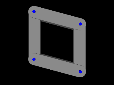
To model a four-bar in ArtiSynth presently requires adding compliance to the hinge joints. An example of this is defined by the demo program
artisynth.demos.tutorial.FourBarLinkage
shown in Figure 3.13. The code for the build() method and a couple of supporting methods is given below:
Two helper methods are used to construct the model: createLink()
(lines 6-17), and createJoint() (lines 23-36). createLink() makes the individual rigid bodies used to build the
linkage: a mesh is produced defining the body’s shape (a box with
rounded ends), and then passed to the
RigidBody
createFromMesh() method which creates the body and sets its
inertia according to a specified density. The body’s pose is then set
so as to center it at ![]() while rotating it about the
while rotating it about the ![]() axis
by the angle deg (in degrees). The completed body is then added to the
MechModel mech and returned.
axis
by the angle deg (in degrees). The completed body is then added to the
MechModel mech and returned.
The second helper method, createJoint(), connects two rigid
bodies (link0 and link1) together using a HingeJoint. Because we know the location of the joint in
body-relative coordinates, it is easier to create the joint using the
transforms ![]() and
and ![]() instead of
instead of ![]() :
: ![]() locates the joint at the top end of link0, at
locates the joint at the top end of link0, at ![]() ,
with the
,
with the ![]() axis parallel to the body’s
axis parallel to the body’s ![]() axis, while
axis, while ![]() similarly locates the joint at the bottom of link1. After the
joint is created and added to the MechModel, its render
properties are set so that its axis is drawn as a blue cylinder.
similarly locates the joint at the bottom of link1. After the
joint is created and added to the MechModel, its render
properties are set so that its axis is drawn as a blue cylinder.
The build() method itself begins by creating a MechModel
and setting damping parameters for the rigid bodies (lines
40-43). Next, createLink() is used to create and store the four
links (lines 46-50), and the left bar is attached to ground by making
it non-dynamic (line 52). The links are then connected together using
joints created by createJoint() (lines 55-59). Finally, uniform
compliance and damping values are set for each of the joint’s
bilateral constraints, using the setCompliance() and setDamping() methods (lines 63-72). Values are set for the first five
constraints, since for a HingeJoint these are the bilateral
constraints. The compliance value of ![]() was found
experimentally to be low enough so as to not cause noticeable
deflections in the joints. Given
was found
experimentally to be low enough so as to not cause noticeable
deflections in the joints. Given ![]() and an
average mass of around
and an
average mass of around ![]() for each link pair,
(3.18) suggests the damping factor of
for each link pair,
(3.18) suggests the damping factor of ![]() . Note that for this example, very similar settings could be
achieved by simply calling
. Note that for this example, very similar settings could be
achieved by simply calling
In principle, we only need to set compliance for the constraints that are redundant, but it can sometimes be difficult to determine exactly which these are. Also, different values are often needed for linear and rotary constraints; that is not necessary here because the links have unit length and so the linear and rotary units have similar scales.
3.4.11 Rendering joints
Most joints provide a means to render themselves in order to provide a graphical representation of their position and configuration. Control over this is achieved by setting various properties in the joint component, including both specialized properties and the standard render properties (Section 4.3) used by all renderable components.
All joints which are subclasses of JointBase support rendering of both their C and D coordinate frames, through the properties drawFrameC, drawFrameD, and axisLength. The first two properties are of the type Renderer.AxisDrawStyle (described in detail in Section 3.2.8), and can be set to LINE or ARROW to enable the coordinate axes to be drawn either as lines or solid arrows. The axisLength property has type double and specifies the length with which the axes are drawn. As with all properties, these properties can be set either in the GUI, or in code using accessor methods supplied by the joint:
Another pair of properties used by several joints is shaftLength and shaftRadius, which specify the length and radius used to draw shaft or axis structures associated with the joint. These are rendered as solid cylinders, using the color indicated by the faceColor rendering property. The default value of both properties is 0; if shaftLength is 0, then the structures are not drawn, while if shaftRadius is 0, a default value proportional to shaftLength is used. For example, to enable rendering of a blue shaft along the rotation axis of a hinge joint, one may use the code fragment
As another example, to enable rendering of a green ball about the center of a spherical joint, one may use the fragment
Specific joints may define additional properties to control how they are rendered.
3.5 Joint components
ArtiSynth supplies a number of basic joints and connectors in the package artisynth.core.mechmodels, the most common of which are described here.
Many of the descriptions are associated with a demonstration model, named XXXJointDemo, where XXX is the joint type. These demos are located in the package artisynth.demos.mech, and can be loaded by selecting All demos > mech > XXXJointDemo from the Models menu. When run, they can be interactively controlled, using either the pull tool (see the section “Pull Manipulation” in the ArtiSynth User Interface Guide), or the interactive control panel. The control panel allows the adjustment of coordinate values and ranges (if supported), some of the render properties, and the different compliance and damping properties (Section 3.4.9). One can inspect the source code for each demo in its .java file located in the folder <ARTISYNTH_HOME>/src/artisynth/demos/mech.
3.5.1 Hinge joint
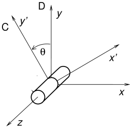 |
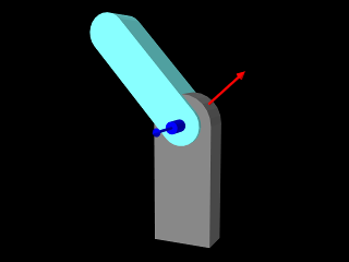 |
The HingeJoint
(Figure 3.14) is a 1 DOF joint that
constrains motion between frames C and D to a simple rotation about
the ![]() axis of D. It implements six constraints and one coordinate
axis of D. It implements six constraints and one coordinate
![]() (Table 3.1), to which the joint transform
(Table 3.1), to which the joint transform
![]() is related by
is related by
|
The value and ranges for ![]() are exported by the properties theta and thetaRange, and the
are exported by the properties theta and thetaRange, and the ![]() coordinate index is
defined by the constant THETA_IDX. For rendering, the
properties shaftLength and shaftRadius control the size of
a shaft drawn about the rotation axis, using the faceColor
rendering property. A demo is provided by
coordinate index is
defined by the constant THETA_IDX. For rendering, the
properties shaftLength and shaftRadius control the size of
a shaft drawn about the rotation axis, using the faceColor
rendering property. A demo is provided by
artisynth.demos.mech.HingeJointDemo.
In addition to the standard constructors described in Section 3.4.3,
creates a hinge joint with a specified origin and ![]() axis direction
for frame D (in world coordinates), and frames C and D coincident.
axis direction
for frame D (in world coordinates), and frames C and D coincident.
| Index | type/name | description |
|---|---|---|
| 0 | bilateral | restricts translation along |
| 1 | bilateral | restricts translation along |
| 2 | bilateral | restricts translation along |
| 3 | bilateral | restricts rotation about |
| 4 | bilateral | restricts rotation about |
| 5 | unilateral | enforces limits on |
| 0 | counter-clockwise rotation of |
3.5.2 Slider joint
 |
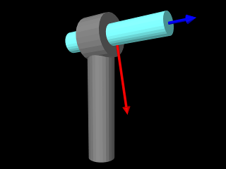 |
The SliderJoint
(Figure 3.15) is a 1 DOF joint
that constrains motion between frames C and D to a simple translation
along the ![]() axis of D. It implements six constraints and one
coordinate
axis of D. It implements six constraints and one
coordinate ![]() (Table 3.2), to which the joint
transform
(Table 3.2), to which the joint
transform ![]() is related by
is related by
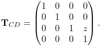 |
The value and ranges for ![]() are exported by the properties z
and zRange, and the
are exported by the properties z
and zRange, and the ![]() coordinate index is defined by the
constant Z_IDX. For rendering, the properties shaftLength and shaftRadius control the size of a shaft drawn
about the sliding axis, using the faceColor rendering property.
A demo is provided by artisynth.demos.mech.SliderJointDemo.
coordinate index is defined by the
constant Z_IDX. For rendering, the properties shaftLength and shaftRadius control the size of a shaft drawn
about the sliding axis, using the faceColor rendering property.
A demo is provided by artisynth.demos.mech.SliderJointDemo.
In addition to the standard constructors described in Section 3.4.3,
creates a slider joint with a specified origin and ![]() axis direction
for frame D (in world coordinates), and frames C and D coincident.
axis direction
for frame D (in world coordinates), and frames C and D coincident.
| Index | type/name | description |
|---|---|---|
| 0 | bilateral | restricts translation along |
| 1 | bilateral | restricts translation along |
| 2 | bilateral | restricts rotation about |
| 3 | bilateral | restricts rotation about |
| 4 | bilateral | restricts rotation about |
| 5 | unilateral | enforces limits on the |
| 0 | translation of |
3.5.3 Cylindrical joint
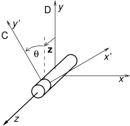 |
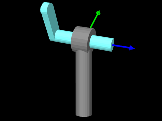 |
The CylindricalJoint
(Figure 3.16) is a 2 DOF
joint that constrains motion between frames C and D to translation and
rotation along and about the ![]() axis of D. It implements six
constraints and two coordinates
axis of D. It implements six
constraints and two coordinates ![]() and
and ![]() (Table 3.3), to which the joint transform
(Table 3.3), to which the joint transform
![]() is related by
is related by
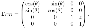 |
The value and ranges for ![]() and
and ![]() are exported by the
properties z, theta, zRange and thetaRange,
and the coordinate indices are defined by the constants Z_IDX
and THETA_IDX. For rendering, the properties shaftLength
and shaftRadius control the size of a shaft drawn about the
sliding/rotation axis, using the faceColor rendering property.
A demo is provided by artisynth.demos.mech.CylindricalJointDemo.
are exported by the
properties z, theta, zRange and thetaRange,
and the coordinate indices are defined by the constants Z_IDX
and THETA_IDX. For rendering, the properties shaftLength
and shaftRadius control the size of a shaft drawn about the
sliding/rotation axis, using the faceColor rendering property.
A demo is provided by artisynth.demos.mech.CylindricalJointDemo.
In addition to the standard constructors described in Section 3.4.3,
creates a cylindrical joint with a specified origin and ![]() axis direction
for frame D (in world coordinates), and frames C and D coincident.
axis direction
for frame D (in world coordinates), and frames C and D coincident.
| Index | type/name | description |
|---|---|---|
| 0 | bilateral | restricts translation along |
| 1 | bilateral | restricts translation along |
| 2 | bilateral | restricts rotation about |
| 3 | bilateral | restricts rotation about |
| 4 | unilateral | enforces limits on the |
| 5 | unilateral | enforces limits on the |
| 0 | translation of |
|
| 1 | rotation of |
3.5.4 Slotted hinge joint
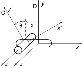 |
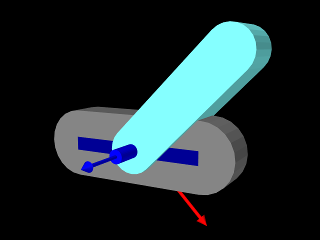 |
The SlottedHingeJoint
(Figure 3.17) is
a 2 DOF joint that constrains motion between frames C and D to
translation along the ![]() axis and rotation about the
axis and rotation about the ![]() axis of D.
It implements six constraints and two coordinates
axis of D.
It implements six constraints and two coordinates ![]() and
and ![]() (Table 3.4), to which the joint
transform
(Table 3.4), to which the joint
transform ![]() is related by
is related by
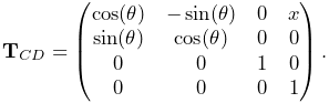 |
(3.19) |
The value and ranges for ![]() and
and ![]() are exported by the
properties x, theta, xRange and thetaRange,
and the coordinate indices are defined by the constants X_IDX
and THETA_IDX. For rendering, the properties shaftLength
and shaftRadius control the size of a shaft drawn about the
rotation axis, while slotWidth and slotDepth control the
width and depth of a slot drawn along the sliding (
are exported by the
properties x, theta, xRange and thetaRange,
and the coordinate indices are defined by the constants X_IDX
and THETA_IDX. For rendering, the properties shaftLength
and shaftRadius control the size of a shaft drawn about the
rotation axis, while slotWidth and slotDepth control the
width and depth of a slot drawn along the sliding (![]() ) axis; both are
drawn using the faceColor rendering property. When rendering the
slot, its bounds along the
) axis; both are
drawn using the faceColor rendering property. When rendering the
slot, its bounds along the ![]() axis are set to xRange by
default. However, this may be too large, particularly if xRange
is unbounded. As an alternate, the property slotRange will be
used instead if its range (i.e., the upper bound minus the lower
bound) exceeds 0. A demo of SlottedHingeJoint is provided by
artisynth.demos.mech.SlottedHingeJointDemo.
axis are set to xRange by
default. However, this may be too large, particularly if xRange
is unbounded. As an alternate, the property slotRange will be
used instead if its range (i.e., the upper bound minus the lower
bound) exceeds 0. A demo of SlottedHingeJoint is provided by
artisynth.demos.mech.SlottedHingeJointDemo.
In addition to the standard constructors described in Section 3.4.3,
creates a slotted hinge joint with a specified origin and ![]() axis direction
for frame D (in world coordinates), and frames C and D coincident.
axis direction
for frame D (in world coordinates), and frames C and D coincident.
| Index | type/name | description |
|---|---|---|
| 0 | bilateral | restricts translation along |
| 1 | bilateral | restricts translation along |
| 2 | bilateral | restricts rotation about |
| 3 | bilateral | restricts rotation about |
| 4 | unilateral | enforces limits on the |
| 5 | unilateral | enforces limits on the |
| 0 | translation of |
|
| 1 | rotation of |
3.5.5 Universal joint
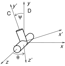 |
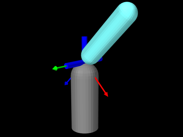 |
| Index | type/name | description |
|---|---|---|
| 0 | bilateral | restricts translation along |
| 1 | bilateral | restricts translation along |
| 2 | bilateral | restricts translation along |
| 3 | bilateral | restricts rotation about the final |
| 4 | unilateral | enforces limits on the roll coordinate |
| 5 | unilateral | enforces limits on the pitch coordinate |
| 0 |
|
first rotation of |
| 1 |
|
second rotation of |
The UniversalJoint
(Figure 3.18) is a 2 DOF joint
that allows C two rotational degrees of freedom with respect to D: a
roll rotation ![]() about D’s
about D’s ![]() axis, followed by a pitch rotation
axis, followed by a pitch rotation ![]() about the rotated
about the rotated ![]() axis. It implements six
constraints and the two coordinates
axis. It implements six
constraints and the two coordinates ![]() and
and ![]() (Table 3.5), to which the joint transform
(Table 3.5), to which the joint transform
![]() is related by
is related by
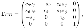 |
where
The value and ranges for ![]() and
and ![]() are exported by the
properties roll, pitch, rollRange and pitchRange, and the coordinate indices are defined by the constants
ROLL_IDX and PITCH_IDX.
are exported by the
properties roll, pitch, rollRange and pitchRange, and the coordinate indices are defined by the constants
ROLL_IDX and PITCH_IDX.
For rendering, the properties shaftLength and shaftRadius control the size of shafts drawn about the roll and pitch axes, while jointRadius specifies the radius of a ball drawn around the origin of D; both are drawn using the faceColor rendering property. It is also possible to add a rendering mesh, using the methods:
If present, the rendering mesh is rendered in the intermediate
frame between D and C, i.e., D rotated about ![]() by
by ![]() .
Rendering is controlled by the face rendering properties (
faceStyle, faceColor, etc.).
.
Rendering is controlled by the face rendering properties (
faceStyle, faceColor, etc.).
A demo is provided by artisynth.demos.mech.UniversalJointDemo.
3.5.6 Skewed universal joint
The SkewedUniversalJoint
(Figure 3.19) is a version of the universal
joint in which the pitch axis is skewed relative to its nominal direction
by an angle ![]() . More precisely, let
. More precisely, let ![]() and
and ![]() be the
be the ![]() and
and
![]() axes of C after the initial roll rotation. For a regular universal
joint, the pitch axis is
axes of C after the initial roll rotation. For a regular universal
joint, the pitch axis is ![]() , whereas for a skewed universal joint it
is
, whereas for a skewed universal joint it
is ![]() rotated by
rotated by ![]() clockwise about
clockwise about ![]() . The joint still has
2 DOF, but the space of allowed rotations is reduced.
. The joint still has
2 DOF, but the space of allowed rotations is reduced.
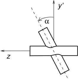 |
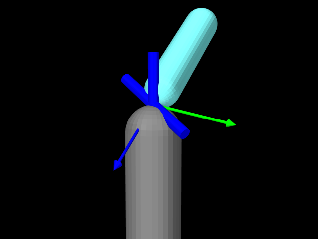 |
The constraints and the coordinates are the same as for the universal
joint, although the expression for ![]() is now more complicated.
With
is now more complicated.
With ![]() ,
, ![]() ,
, ![]() , and
, and ![]() defined as for the universal
joint,
defined as for the universal
joint, ![]() is given by
is given by
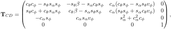 |
where
Rendering is controlled using the properties shaftLength, shaftRadius and jointRadius in the same way as for the UniversalJoint. A demo is provided by calling artisynth.demos.mech.UniversalJointDemo with the model arguments -skew <angDeg>, where <angDeg> is the desired skew angle in degrees.
Constructors for skewed universal joints take the standard forms described in Section 3.4.3, with an additional argument at the end indicating the skew angle:
In addition, the constructor
creates a skewed universal joint specifying the origin of frame D together with the directions of the roll and pitch axes (in world coordinates). Frames C and D are coincident and the skew angle is inferred from the angle between the axes.
3.5.7 Gimbal joint
 |
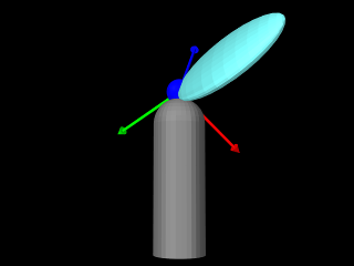 |
The GimbalJoint
(Figure 3.20) is a 3 DOF spherical joint that anchors
the origins of C and D together but otherwise allows C complete
rotational freedom. The rotational degrees of freedom are
parameterized by three roll-pitch-yaw angles, denoted by
![]() , which define a rotation
, which define a rotation ![]() about D’s
about D’s ![]() axis, followed by a second rotation
axis, followed by a second rotation ![]() about the rotated
about the rotated ![]() axis, followed by a third rotation
axis, followed by a third rotation ![]() about the final
about the final ![]() axis.
It implements six constraints and the three coordinates
axis.
It implements six constraints and the three coordinates
![]() (Table 3.6), to which the
joint transform
(Table 3.6), to which the
joint transform ![]() is related by
is related by
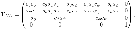 |
where
The value and ranges for ![]() are exported by the
properties roll, pitch, yaw, rollRange, pitchRange, and yawRange, and the coordinate indices are
defined by the constants ROLL_IDX, PITCH_IDX, and YAW_IDX. For rendering, the property jointRadius specifies the
radius of a ball drawn around the origin of D, using the faceColor rendering property. A demo is provided by artisynth.demos.mech.GimbalJointDemo.
are exported by the
properties roll, pitch, yaw, rollRange, pitchRange, and yawRange, and the coordinate indices are
defined by the constants ROLL_IDX, PITCH_IDX, and YAW_IDX. For rendering, the property jointRadius specifies the
radius of a ball drawn around the origin of D, using the faceColor rendering property. A demo is provided by artisynth.demos.mech.GimbalJointDemo.
In addition to the standard constructors described in Section 3.4.3,
creates a gimbal joint with a specified origin for frame D (in world coordinates), and frames C and D coincident and world aligned.
The constraints implementing GimbalJoint are designed so that it is immune to gimbal lock, in which a degree of freedom is lost when
. However, the coordinate values themselves are not immune to this singularity, and neither are the unilateral constraints which enforce limits on their values. Therefore, if coordinate limits are implemented, the joint should be deployed so as to avoid pitch values near
.
| Index | type/name | description |
|---|---|---|
| 0 | bilateral | restricts translation along |
| 1 | bilateral | restricts translation along |
| 2 | bilateral | restricts translation along |
| 3 | unilateral | enforces limits on the roll coordinate |
| 4 | unilateral | enforces limits on the pitch coordinate |
| 5 | unilateral | enforces limits on the yaw coordinate |
| 0 |
|
first rotation of |
| 1 |
|
second rotation of |
| 2 |
|
third rotation of |
3.5.8 Spherical joint
 |
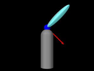 |
The SphericalJoint (Figure 3.21) is a 3 DOF spherical joint that, like GimbalJoint, anchors the origins of C and D together but otherwise allows C complete rotational freedom. SphericalJoint does not implement any coordinates, and so is conceptually more like a ball joint. However, it does provide two choices for limiting its rotation:
-
•
A limit on the tilt angle
 between
the
between
the  axes of D and C, such that
(3.20) This is intended to emulate the limit imposed by a ball joint socket.
-
•
A limit on the total rotation, defined as follows: Let
 be the axis-angle representation of the rotation matrix of
  ,
normalized such that
,
normalized such that  and
and  , and let
 be a three-vector giving maximum rotation angles with
 ,
,  , and components. Then
  is constrained by
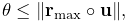
(3.21) where
 denotes the element-wise product. If the components of
are set to a uniform value
denotes the element-wise product. If the components of
are set to a uniform value  , this
simplifies to
, this
simplifies to  .
.
These limits can be enabled by setting the joint’s properties isTiltLimited and isRotationLimited, respectively, where
enabling one disables the other. The limit values ![]() and
and ![]() are managed using the properties maxTilt and
maxRotation, and setting either automatically enables tilt or
rotation limiting, as appropriate. Finally, the tilt angle
are managed using the properties maxTilt and
maxRotation, and setting either automatically enables tilt or
rotation limiting, as appropriate. Finally, the tilt angle ![]() can
be queried using the (read-only) tilt property. For rendering,
the property jointRadius specifies the radius of a ball drawn
around the origin of D, using the faceColor rendering
property. A demo of the SphericalJoint is provided by artisynth.demos.mech.SphericalJointDemo.
can
be queried using the (read-only) tilt property. For rendering,
the property jointRadius specifies the radius of a ball drawn
around the origin of D, using the faceColor rendering
property. A demo of the SphericalJoint is provided by artisynth.demos.mech.SphericalJointDemo.
In addition to the standard constructors described in Section 3.4.3,
creates a spherical joint with a specified origin for frame D (in world coordinates), and frames C and D coincident and world aligned.
One should use the rotation limit with some caution, as the orientations which it prohibits can be somewhat hard to predict, particularly when
| Index | type/name | description |
|---|---|---|
| 0 | bilateral | restricts translation along |
| 1 | bilateral | restricts translation along |
| 2 | bilateral | restricts translation along |
| 3 | unilateral | enforces either the “tilt” or “rotation” limits |
3.5.9 Planar joint
 |
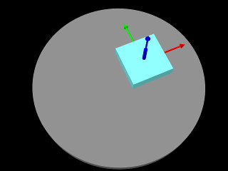 |
The PlanarJoint
(Figure 3.22) is a 3 DOF
joint that constrains C to translation in the ![]() -
-![]() plane
and rotation about the
plane
and rotation about the ![]() axis of D. It implements six
constraints and three coordinates
axis of D. It implements six
constraints and three coordinates ![]() ,
, ![]() and
and ![]() (Table 3.8), to which the joint transform
(Table 3.8), to which the joint transform
![]() is related by
is related by
 |
The value and ranges for ![]() ,
, ![]() and
and ![]() are exported by the
properties x, y, theta, xRange, yRange
and thetaRange, and the coordinate indices are defined by the
constants X_IDX, Y_IDX and THETA_IDX.
A planar joint can be rendered as a square centered on the origin
of D, using face rendering properties and with a size given by the
planeSize property. For example,
are exported by the
properties x, y, theta, xRange, yRange
and thetaRange, and the coordinate indices are defined by the
constants X_IDX, Y_IDX and THETA_IDX.
A planar joint can be rendered as a square centered on the origin
of D, using face rendering properties and with a size given by the
planeSize property. For example,
will cause joint to be drawn as a light gray square with size 5.0. The default value of planeSize is 0, so drawing the plane is disabled by default. Also, the default faceStyle rendering property for PlanarConnector is set to FRONT_AND_BACK, so that the plane (when drawn) can be seen from both sides. A shaft about the rotation axis can also be drawn, as controlled by the properties shaftLength and shaftRadius and using the faceColor rendering property. A demo is provided by artisynth.demos.mech.PlanarJointDemo.
In addition to the standard constructors described in Section 3.4.3,
creates a planar joint with a specified origin and ![]() axis direction
for frame D (in world coordinates), and frames C and D coincident.
axis direction
for frame D (in world coordinates), and frames C and D coincident.
| Index | type/name | description |
|---|---|---|
| 0 | bilateral | restricts translation along |
| 1 | bilateral | restricts rotation about |
| 2 | bilateral | restricts rotation about |
| 3 | unilateral | enforces limits on the |
| 4 | unilateral | enforces limits on the |
| 5 | unilateral | enforces limits on the |
| 0 | translation of |
|
| 1 | translation of |
|
| 2 | rotation of |
3.5.10 Planar translation joint
 |
| Index | type/name | description |
|---|---|---|
| 0 | bilateral | restricts translation along |
| 1 | bilateral | restricts rotation about |
| 2 | bilateral | restricts rotation about |
| 3 | bilateral | restricts rotation about |
| 4 | unilateral | enforces limits on the |
| 5 | unilateral | enforces limits on the |
| 0 | translation of |
|
| 1 | translation of |
The PlanarTranslationJoint
(Figure 3.23) is a 2 DOF joint
that is the same as the planar joint without rotation:
C is restricted to translation in the ![]() -
-![]() plane of D.
It implements six
constraints and two coordinates
plane of D.
It implements six
constraints and two coordinates ![]() and
and ![]() (Table 3.9), to which the joint transform
(Table 3.9), to which the joint transform
![]() is related by
is related by
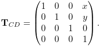 |
The value and ranges for ![]() and
and ![]() are exported by the properties
x, y, xRange and yRange, and the coordinate
indices are defined by the constants X_IDX and Y_IDX. A
planar translation joint can be rendered as a square centered on the
origin of D, using face rendering properties and with a size given by
the planeSize property, in the same way as described for PlanarJoint. A demo is provided by artisynth.demos.mech.PlanarJointDemo.
are exported by the properties
x, y, xRange and yRange, and the coordinate
indices are defined by the constants X_IDX and Y_IDX. A
planar translation joint can be rendered as a square centered on the
origin of D, using face rendering properties and with a size given by
the planeSize property, in the same way as described for PlanarJoint. A demo is provided by artisynth.demos.mech.PlanarJointDemo.
3.5.11 Ellipsoid joint
The EllipsoidJoint is a 4 DOF joint that provides similar functionality to the ellipsoidal and scapulothoracic joints available in OpenSim. It allows the origin of C to slide around on the surface of an ellipsoid centered on the origin of D, together with two additional rotational degrees of freedom.
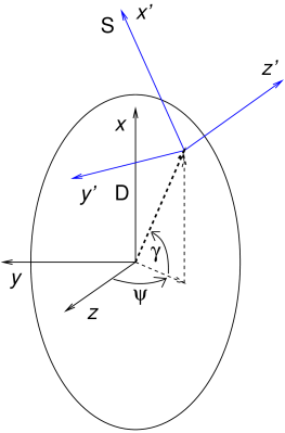 |
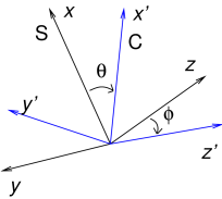 |
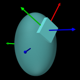 |
The joint kinematics is easiest to describe in terms of an
intermediate frame S whose origin lies on the ellipsoid surface,
with its position controlled by two coordinates: a longitude
angle ![]() , and a latitude angle
, and a latitude angle ![]() (Figure
3.24, left). Frame C has the same origin as
S, with two additional coordinates,
(Figure
3.24, left). Frame C has the same origin as
S, with two additional coordinates, ![]() and
and ![]() which allow it
to rotate about S (Figure 3.24, middle). If the
transform
which allow it
to rotate about S (Figure 3.24, middle). If the
transform ![]() from S to D and the (rotational-only) transform
from S to D and the (rotational-only) transform
![]() from C to S are given by
from C to S are given by
then ![]() is given by
is given by
The six constraints and four coordinates of the ellipsoidal joint are described in table 3.10.
| Index | type/name | description |
| 0 | bilateral | restricts C to the ellipsoid surface and limits rotation |
| 1 | bilateral | restricts C to the ellipsoid surface and limits rotation |
| 2 | unilateral | enforces limits on the |
| 3 | unilateral | enforces limits on the |
| 4 | unilateral | enforces limits on the |
| 5 | unilateral | enforces limits on the |
| 0 | longitude angle for origin of S (and C) on the ellipsoid | |
| 1 | latitude angle for origin of S (and C) on the ellipsoid | |
| 2 | first rotation of C about the |
|
| 3 | second rotation of C about rotated |
For frame S, if ![]() ,
, ![]() and
and ![]() are the ellipsoid semi-axis lengths
for the
are the ellipsoid semi-axis lengths
for the ![]() ,
, ![]() , and
, and ![]() axes, and
axes, and ![]() ,
, ![]() ,
, ![]() ,
and
,
and ![]() are the cosines and sines of
are the cosines and sines of ![]() and
and ![]() , we
can show that
, we
can show that
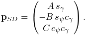 |
For the orientation of S, the ![]() axis of S is parallel to the surface
normal and the
axis of S is parallel to the surface
normal and the ![]() axis is parallel to the tangent direction imparted
by the latitudinal velocity
axis is parallel to the tangent direction imparted
by the latitudinal velocity ![]() . That means
. That means ![]() and
and ![]() axes are parallel to the direction vectors
axes are parallel to the direction vectors ![]() and
and ![]() given by
given by
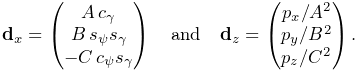 |
(3.22) |
The columns of ![]() are then given by the normalized values
of
are then given by the normalized values
of ![]() ,
, ![]() , and
, and ![]() , respectively.
, respectively.
The rotation ![]() is formed by a rotation
is formed by a rotation ![]() about the
about the ![]() axis, followed by a rotation of
axis, followed by a rotation of ![]() about the new
about the new ![]() axis.
Letting
axis.
Letting ![]() ,
, ![]() ,
, ![]() , and
, and ![]() be the cosines and sines of
be the cosines and sines of
![]() and
and ![]() , we then have
, we then have
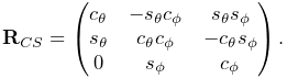 |
If desired, the ![]() rotation can instead be performed about a
modified axis
rotation can instead be performed about a
modified axis ![]() that makes an angle
that makes an angle ![]() with respect to
with respect to ![]() in the
in the ![]() -
-![]() plane.
plane. ![]() is controlled by the joint’s alpha
property (default value
is controlled by the joint’s alpha
property (default value ![]() ) and corresponds to the “winging” angle
of the OpenSim scapulothoracic joint. If
) and corresponds to the “winging” angle
of the OpenSim scapulothoracic joint. If ![]() ,
,
![]() takes the more complex form
takes the more complex form
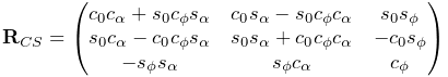 |
where ![]() ,
, ![]() ,
, ![]() , and
, and ![]() are the cosines and sines of
are the cosines and sines of
![]() and
and ![]() , respectively.
, respectively.
Within an EllipsoidJoint, the values and ranges for ![]() ,
,
![]() ,
, ![]() and
and ![]() are exported by the properties longitude, latitude, theta, phi, longitudeRange, latitudeRange, thetaRange, and phiRange, and the coordinate indices are defined by the constants
LONGITUDE_IDX, LATITUDE_IDX, THETA_IDX, and PHI_IDX. For rendering, the property drawEllipsoid specifies
whether the ellipsoid surface should be drawn; if true, it will
be drawn using the joint’s face rendering properties. A demo is
provided by artisynth.demos.mech.EllipsoidJointDemo.
are exported by the properties longitude, latitude, theta, phi, longitudeRange, latitudeRange, thetaRange, and phiRange, and the coordinate indices are defined by the constants
LONGITUDE_IDX, LATITUDE_IDX, THETA_IDX, and PHI_IDX. For rendering, the property drawEllipsoid specifies
whether the ellipsoid surface should be drawn; if true, it will
be drawn using the joint’s face rendering properties. A demo is
provided by artisynth.demos.mech.EllipsoidJointDemo.
Ellipsoid joints can be created with the following constructors:
The first of these creates a joint that is not attached to any
bodies; attachment can be done later using one of the setBodies() methods. Its semi-axis lengths are given by A,
B, and C, its ![]() angle is given by alpha, and
the argument openSimCompatible, if true, makes the joint
kinematics compatible with OpenSim (Section 3.5.11.1).
The second constructor creates a joint and then attaches it to rigid
bodies rbodyA and rbodyB, with the specified
angle is given by alpha, and
the argument openSimCompatible, if true, makes the joint
kinematics compatible with OpenSim (Section 3.5.11.1).
The second constructor creates a joint and then attaches it to rigid
bodies rbodyA and rbodyB, with the specified ![]() and
and
![]() transformations. The third constructor creates a joint and
attaches it to connectable bodies cbodyA and cbodyB, with
the locations of the C and D frames specified in world coordinates by
TCW and TDW.
transformations. The third constructor creates a joint and
attaches it to connectable bodies cbodyA and cbodyB, with
the locations of the C and D frames specified in world coordinates by
TCW and TDW.
Unlike in many joints,
. That is because the origin of C must lie on the ellipsoid surface, and since D is at the center of the ellipsoid,
but
.
3.5.11.1 OpenSim compatibility
The openSimCompatible argument in some of the joint’s
constructors makes the kinematics compatible with the ellipsoidal
joint used by OpenSim. This means that ![]() is computed
differently: in OpenSim, instead of
using (3.22), the
is computed
differently: in OpenSim, instead of
using (3.22), the ![]() and
and ![]() axis directions of
axis directions of
![]() are computed using
are computed using
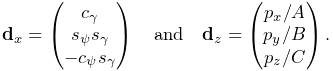 |
(3.23) |
In particular, this means that the ![]() axis is only approximately
parallel to the ellipsoid surface normal.
axis is only approximately
parallel to the ellipsoid surface normal.
In OpenSim, the axes of the C frame of both the ellipsoid and scapulothoracic joints are oriented differently than those of the ArtiSynth joint: they are rotated by
about
and
3.5.12 Solid joint
The SolidJoint
is a 0 DOF joint that rigidly constrains C to D. It
implements six constraints and no coordinates
(Table 3.11) and the resulting ![]() is the
identity.
is the
identity.
There aren’t normally many uses for solid joints. If one wishes to create a complex rigid body by joining together a variety of shapes, this can be done more efficiently by making these shapes mesh components of a single rigid body (Section 3.2.9).
| Index | type/name | description |
|---|---|---|
| 0 | bilateral | restricts translation along |
| 1 | bilateral | restricts translation along |
| 2 | bilateral | restricts translation along |
| 3 | bilateral | restricts rotation about |
| 4 | bilateral | restricts rotation about |
| 5 | bilateral | restricts rotation about |
3.5.13 Planar Connector
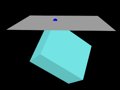 |
| Index | type/name | description |
|---|---|---|
| 0 | bilateral or unilateral | restricts translation along |
The PlanarConnector
(Figure 3.25) is a 5 DOF connector that attaches
the origin of C to the ![]() -
-![]() plane of D. C is completely free to
rotate, and to translate within the
plane of D. C is completely free to
rotate, and to translate within the ![]() -
-![]() plane. Only motion in the
plane. Only motion in the
![]() direction is restricted. PlanarConnector implements one
constraint and has no coordinates
(Table 3.12).
direction is restricted. PlanarConnector implements one
constraint and has no coordinates
(Table 3.12).
A PlanarConnector constrains a point on body A (located at the
origin of C) to move within a plane on body B. Several planar
connectors can be employed to constrain body motions in more
complicated ways, although one must be careful to avoid
overconstraining the system. The connector can also be configured to
function unilaterally, via its unilateral property, in
which case the point is constrained to lie in the half-space defined by
![]() with respect to D. Several unilateral PlanarConnectors
can therefore be used to implement a cheap and approximate collision
mechanism with fixed collision points.
with respect to D. Several unilateral PlanarConnectors
can therefore be used to implement a cheap and approximate collision
mechanism with fixed collision points.
When set to function unilaterally, overconstraining the system is not an issue because of the way in which ArtiSynth solves unilateral constraints.
A planar connector can be rendered as a square centered on the origin of D, using face rendering properties and with a size given by the planeSize property. The point attached to A can also be rendered using point rendering properties. For example,
will cause connector to be drawn as a light gray square with size 5, and for the point on body A to be drawn as a blue sphere with radius 0.1. The default value of planeSize is 0, so drawing the plane is disabled by default. Also, the default faceStyle rendering property for PlanarConnector is set to FRONT_AND_BACK, so that the plane (when drawn) can be seen from both sides.
Constructors for the PlanarConnector include
where pCA gives the connection point of body A with respect to frame A, TDB gives the transform from frame D to frame B, and TDW gives the transform from frame D to world.
3.5.14 Segmented Planar Connector
 |
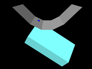 |
| Index | type/name | description |
|---|---|---|
| 0 | bilateral or unilateral | restricts translation normal to the surface |
The SegmentedPlanarConnector
(Figure 3.26) is a 5 DOF connector that
generalizes PlanarConnector to a piecewise linear surface, to
which the origin of ![]() is constrained while
is constrained while ![]() is otherwise
completely free to rotate. The surface is specified by a sequence of
2D points defining a piecewise linear curve in the
is otherwise
completely free to rotate. The surface is specified by a sequence of
2D points defining a piecewise linear curve in the ![]() -
-![]() plane of D
(Figure 3.26, left). This curve does not
need to be a function; the segment nearest to C is the one used to
enforce the constraint at any given time. The surface has infinite
extent and is extrapolated beyond the first and last segments. It
implements one constraint and has no coordinates (Table
3.13).
plane of D
(Figure 3.26, left). This curve does not
need to be a function; the segment nearest to C is the one used to
enforce the constraint at any given time. The surface has infinite
extent and is extrapolated beyond the first and last segments. It
implements one constraint and has no coordinates (Table
3.13).
By appropriate choice of segments, a SegmentedPlanarConnector
can approximate any surface defined by a curve in the ![]() -
-![]() plane.
As with PlanarConnector, it can also be configured as
unilateral, constraining the origin of
plane.
As with PlanarConnector, it can also be configured as
unilateral, constraining the origin of ![]() to lie on the side of the
surface defined by the normal vectors
to lie on the side of the
surface defined by the normal vectors ![]() of each segment
of each segment ![]() . If
. If
![]() and
and ![]() are the points in the
are the points in the ![]() -
-![]() plane defining the
plane defining the
![]() -th segment, and
-th segment, and ![]() is the
is the ![]() axis unit vector, then
axis unit vector, then ![]() is given by
is given by
| (3.24) |
The properties controlling the rendering of a segmented planar
connector are the same as for a planar connector, with each of the
individual plane segments drawn as a rectangle whose length along the
![]() axis is controlled by planeSize.
axis is controlled by planeSize.
Constructors for a SegmentedPlanarConnector are analogous to those used for PlanarConnector,
where segs is an additional argument of type double[]
giving the 2D coordinates defining the segments in the ![]() -
-![]() plane.
plane.
3.5.15 Legacy Joints
ArtiSynth maintains three legacy joints for compatibility with earlier software:
-
•
RevoluteJoint is identical to the HingeJoint, except that its coordinate
is oriented clockwise about the axis
instead of counter-clockwise. Rendering is also done
differently, with shafts about the rotation axis drawn using
line rendering properties. -
•
RollPitchJoint is identical to the UniversalJoint, except that its roll-pitch coordinates
 are computed with
respect to the rotation
are computed with
respect to the rotation  from frame D to C, instead of the
rotation
from frame D to C, instead of the
rotation  from frame C to D. Rendering is also done
differently, with shafts along the roll and pitch axes drawn
using line rendering properties, and the ball around the
origin of D drawn using point rendering properties.
from frame C to D. Rendering is also done
differently, with shafts along the roll and pitch axes drawn
using line rendering properties, and the ball around the
origin of D drawn using point rendering properties. -
•
SphericalRpyJoint is identical to the GimbalJoint, except that its roll-pitch-yaw coordinates
 are computed with
respect to the rotation from frame D to C, instead of the
rotation from frame C to D. Rendering is also done
differently, with the ball around the origin of D drawn using point
rendering properties.
are computed with
respect to the rotation from frame D to C, instead of the
rotation from frame C to D. Rendering is also done
differently, with the ball around the origin of D drawn using point
rendering properties.
3.5.16 Example: A multijointed arm
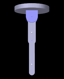 |
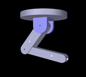 |
The example model
artisynth.demos.tutorial.MultiJointedArm
shows two links connected by universal and hinge joints to form a 3 DOF robot-like arm. The model class definition, excluding the import directives, is shown here:
Line 3 uses getSourceRelativePath() to locate the geometry folder
relative to the model’s source folder and lines 4-5 define some constants. The
build() method begins by creating and adding a MechModel,
specifying a standard inertial damping of 1, as well as a rotary damping value
to reduce spinning of the first joint about the ![]() axis. The class member
variable myMech is used to store a reference to the MechModel so
that it is available to subclasses.
axis. The class member
variable myMech is used to store a reference to the MechModel so
that it is available to subclasses.
A FixedMeshBody is used to illustrate a mounting plate (lines 15-21);
this is purely decorative and has no dynamic purpose. The links and joints are
then created and assembled in the configuration shown in
Figure 3.27 (left). The first link, link0, is
created from a rounded-box mesh, and then repositioned to align vertically
along the ![]() axis under the mounting plate (lines 23-31). The link is then
attached to ground, just below the mounting plate, using a 2 DOF universal
joint (lines 33-42), with a rendering mesh added to illustrate a mounting
bracket and a range limit of
axis under the mounting plate (lines 23-31). The link is then
attached to ground, just below the mounting plate, using a 2 DOF universal
joint (lines 33-42), with a rendering mesh added to illustrate a mounting
bracket and a range limit of ![]() set on the roll angle. (Note that
similar physics could be achieved with two hinge joints and an additional
link.) The second link, link1, is then also created from a rounded-box
mesh and repositioned vertically along the
set on the roll angle. (Note that
similar physics could be achieved with two hinge joints and an additional
link.) The second link, link1, is then also created from a rounded-box
mesh and repositioned vertically along the ![]() axis under link0 (lines
41-52), to which it is attached using a hinge joint (lines 54-60).
axis under link0 (lines
41-52), to which it is attached using a hinge joint (lines 54-60).
After the linkage has been assembled, some marker points are added to the links (lines 62-67), and the linkage is repositioned by setting some of the joint coordinates (lines 70-72) to assume the configuration shown in Figure 3.27 (right). Finally, some additional render properties are set (lines 73-78).
To run this example in ArtiSynth, select All demos > tutorial > MultiJointedArm from the Models menu. The model should load and initially appear as in Figure 3.27. Running the model will cause the links to fall under gravity. Forces can also be interactively applied using the pull tool (see the section “Pull Manipulation” in the ArtiSynth User Interface Guide).
3.6 Setting joint coordinates
As mentioned above, joint coordinate values are not fundamental representations of system state as they are in some other multibody systems, such as OpenSim. This means that they need to be inferred from the relative poses of the bodies connected by their joints. It also means that when setting the values for one or more coordinates, the poses of the surrounding bodies must be updated. In addition, it is usually necessary to also update the wrap paths of any MultiPointSpring or MultiPointMuscle components attached to the bodies. This functionality is provided by the CoordinateSetter class.
3.6.1 Using the CoordinateSetter
A CoordinateSetter is associated with a MechModel and can be created as follows:
A MechModel also maintains its own coordinate setter, which can be obtained as follows:
Once instantiated or obtained, the setter can be used to set coordinate values while ensuring that surrounding body poses and spring/muscle wrap surfaces are updated appropriately. It also handles situations involving closed kinematic chains where not all coordinate values are independent. Coordinate values can be set individually via the following methods:
| SetStatus setCoordinate ( JointCoordinateHandle handle, double value) |
Set coordinate described by handle to value (in radians for rotary coordinates). |
| SetStatus setCoordinate ( JointBase joint, int cidx, double value) |
Set coordinate described by joint and cidx to value (in radians for rotary coordinates). |
| SetStatus setCoordinateDeg ( JointCoordinateHandle handle, double value) |
Set coordinate to described by handle value (in degrees for rotary coordinates). |
| SetStatus setCoordinateDeg ( JointBase joint, int cidx, double value) |
Set coordinate described by joint and cidx to value (in degrees for rotary coordinates). |
Coordinates can be specified using either a JointCoordinateHandle handle (Section 3.4.7), or their joint and its index within it. Each method returns a CoordinateSetter.SetStatus to indicate the success of the operation. For open kinematic chains, coordinate setting always succeeds, but within a closed kinematic chain (Section 3.6.2) not all coordinates are independent and therefore some set operations may fail. All set requests are clipped to the coordinate’s range, if applicable.
Several coordinates can also be set simultaneously, using
| void request ( JointCoordinateHandle handle, double value) |
Queue request to set coordinate described by handle to value (in radians for rotary coordinates). |
| void request ( JointBase joint, int cidx, double value) |
Queue request to set coordinate described by joint and cidx to value (in radians for rotary coordinates). |
| void requestDeg ( JointCoordinateHandle handle, double value) |
Queue request to set coordinate described by handle to value (in degrees for rotary coordinates). |
| void requestDeg ( JointBase joint, int cidx, double value) |
Queue request to set coordinate described by joint and cidx to value (in degrees for rotary coordinates). |
| SetStatus setCoordinates() |
Apply all set requests. |
| void clearRequests() |
Clear all outstanding set requests. |
The request() methods queue specific coordinate set requests, and then setCoordinates() attempts to satisfy them all simultaneously, returning a CoordinateSetter.SetStatus to indicate its success.
As an example, the following code could be used to set coordinates at the end of the build() method for the multijointed arm example of Section 3.5.16:
Joint coordinates can also be set interactively in the GUI using a coordinate panel (Section 5.1.4), and the CoordinatePanel class provides access to its underlying CoordinateSetter and convenience wrappers for some of its methods.
3.6.2 Coordinates in closed kinematic chains
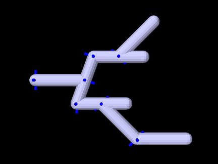
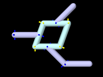
Coordinates can be assigned arbitrarily for any joint which is part of an open kinematic chain forming a linear or tree-shaped structure (Figure 3.28). However, this is not true for closed kinematic chains, in which joints (and possibly other constraints) connect a set of bodies into a loop (Figure 3.29). Closed chains also present challenges for simulation, as discussed in Section 3.4.10.
The formation of kinematic loops reduces the number of degrees of freedom and reduces the number of joint coordinates which can be set independently, in a manner that depends on the joints and connection topology. For the joints in the loop of Figure 3.29, only two of the eight coordinates can be set independently. It is possible (and typical) for a kinematic loop to be embedded within a kinematic structure that is otherwise open, and this is true in Figure 3.29, where the non-loop joints (shown in dark blue) can still be positioned arbitrarily.
When using a CoordinateSetter to set several coordinates at once within a kinematic loop, the request will only partially succeed if the number of coordinates being set exceeds the number of independent coordinates. Requests may also fail if some of the dependent coordinates encounter a range limit. For example, the four bar linkage of Section 3.4.10 has four joints but only one degree of freedom, and so trying to set more than one coordinate will fail, which can be verified by checking the status object returned by setCoordinates():
In general, set requests result in a coordinate either being free (and therefore set to the requested value), dependent (on other coordinate values), or limited (independent but limited because of singularities or dependent coordinate joint limits). Also, very occasionally, if the linkage is near a kinematic singularity, the solver may fail to converge and no coordinates will be set exactly as requested.
SetStatus supplies a number of methods to query coordinate set status, including:
| int numCoordinates() |
Number of coordinates requested to be set. |
|---|---|
| List<JointCoordinateHandle> getCoordinates() |
Query the coordinates requested to be set. |
| boolean converged() |
Queries if the solve converged. |
| int numFree() |
Number of coordinates that are free. |
| boolean isFree (JointCoordinateHandle handle) |
Queries if a coordinate is free. |
| int numFree() |
Number of coordinates that are limited. |
| boolean isLimited (JointCoordinateHandle handle) |
Queries if a coordinate is limited. |
| int numDependent() |
Number of coordinates that are dependent. |
| boolean isDependent (JointCoordinateHandle handle) |
Queries if a coordinate is dependent. |
3.7 Frame springs
Another way to connect two rigid bodies together is to use a frame spring, which is a six dimensional spring that generates restoring forces and moments between coordinate frames.
3.7.1 Frame spring coordinate frames
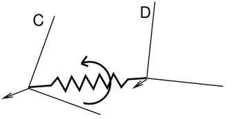
The basic idea of a frame spring is shown in Figure
3.30. It generates restoring forces and moments on
two frames C and D which are a function of ![]() and
and ![]() (the spatial velocity of frame D with respect to frame C).
(the spatial velocity of frame D with respect to frame C).
Decomposing forces into stiffness and damping terms, the force
![]() and moment
and moment ![]() acting on C can be expressed as
acting on C can be expressed as
| (3.24) |
where the translational and rotational forces ![]() ,
, ![]() ,
,
![]() , and
, and ![]() are general functions of
are general functions of ![]() and
and
![]() .
.
The forces acting on D are equal and opposite, so that
| (3.25) |
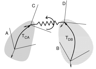
If frames C and D are attached to a pair of rigid bodies A and B, then
a frame spring can be used to connect them in a manner analogous to a
joint. As with joints, C and D generally do not coincide with the body
frames, and are instead offset from them by fixed transforms ![]() and
and ![]() (Figure 3.31).
(Figure 3.31).
For historical reasons, the default behavior for frame springs is to base the restoring forces on
and
, as per (3.24). However, it may be more convenient to instead use
and compute the force
and moment
acting on frame D:
(3.26) For example, using
3.7.2 Frame materials
The restoring forces (3.24) generated in a frame spring depend on the frame material associated with the spring. Frame materials are defined in the package artisynth.core.materials, and are subclassed from FrameMaterial. The most basic type of material is a LinearFrameMaterial, in which the restoring forces are determined from
where ![]() gives the small angle approximation of the
rotational components of
gives the small angle approximation of the
rotational components of ![]() with respect to the
with respect to the ![]() ,
, ![]() , and
, and
![]() axes, and
axes, and
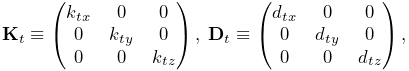 |
||
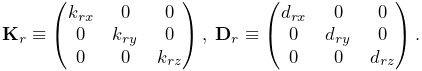 |
are the stiffness and damping matrices. The diagonal values defining
each matrix are stored in the 3-dimensional vectors ![]() ,
, ![]() ,
,
![]() , and
, and ![]() which are exposed as the stiffness, rotaryStiffness, damping, and rotaryDamping properties of
the material. Each of these specifies stiffness or damping values
along or about a particular axis. Specifying different values for
different axes will result in anisotropic behavior.
which are exposed as the stiffness, rotaryStiffness, damping, and rotaryDamping properties of
the material. Each of these specifies stiffness or damping values
along or about a particular axis. Specifying different values for
different axes will result in anisotropic behavior.
Other frame materials offering nonlinear behavior may be defined in artisynth.core.materials.
3.7.2.1 PowerFrameMaterial
A useful alternative to LinearFrameMaterial is PowerFrameMaterial, which computes restoring forces along each of the translational and rotational directions according to a power law of the form
| (3.27) |
where ![]() is a stiffness,
is a stiffness, ![]() is displacement, and
is displacement, and ![]() is an exponent
in the range
is an exponent
in the range ![]() . It is also possible to specify both upper and
lower deadbands,
. It is also possible to specify both upper and
lower deadbands, ![]() and
and ![]() , such that if
, such that if ![]() is the true
displacement,
is the true
displacement, ![]() is computed according to
is computed according to
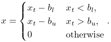 |
(3.28) |
PowerFrameMaterial effects the same damping behavior as LinearFrameMaterial.
If rotational deadbands are specified, the rotational displacement may be large
enough that the small angle approximation used for LinearFrameMaterial no longer applies. Therefore, rotational displacements are
computed as the three x-y-z Tait-Bryan angles of ![]() . The use of
these finite displacement angles introduces a coupling such that if
. The use of
these finite displacement angles introduces a coupling such that if ![]() is
the nominal moment produced by applying (3.27) and
(3.28) to each of the
three rotational angles, the actual resulting moment
is
the nominal moment produced by applying (3.27) and
(3.28) to each of the
three rotational angles, the actual resulting moment ![]() is
is
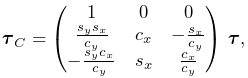 |
(3.29) |
where ![]() ,
, ![]() ,
, ![]() ,
, ![]() are the sines and cosines of the x and y
rotations. The coupling is associated with the non-commutativity of rotations and
the fact that the x-y-z angles have a singularity when the y rotation
approaches
are the sines and cosines of the x and y
rotations. The coupling is associated with the non-commutativity of rotations and
the fact that the x-y-z angles have a singularity when the y rotation
approaches ![]() . This appears as the division by
. This appears as the division by ![]() in
(3.29), and so care should be taken to avoid such
orientations.
in
(3.29), and so care should be taken to avoid such
orientations.
The parameters controlling the behavior of PowerFrameMaterial can be set independently for each of the six translational and rotational displacements, using the following properties, each of which is described by a three-vector:
| Property | Description | |
|---|---|---|
| stiffness | translational stiffness | |
| exponents | translational exponents | |
| upperDeadband | upper deadband for translations | |
| lowerDeadband | lower deadband for translations | |
| damping | translational damping | |
| rotaryStiffness | rotational stiffness | |
| rotaryExponents | rotational exponents | |
| upperRotaryDeadband | upper deadband for rotations | |
| lowerRotaryDeadband | lower deadband for rotations | |
| rotaryDamping | rotational damping |
Each of these has a default value of ![]() , except for the exponents,
which have a default value of
, except for the exponents,
which have a default value of ![]() .
.
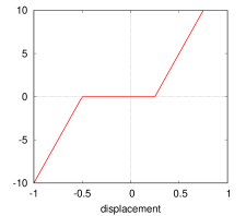 |
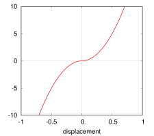 |
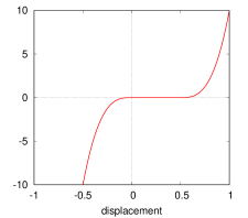 |
If used with exponents of 1 and no deadbands, PowerFrameMaterial behaves
like LinearFrameMaterial with finite rotation displacements. Otherwise,
Figure 3.32 illustrates some of the force-displacement
curves that can be produced. Using a power ![]() (rightmost panels) has the
advantage of producing a curve that is differentiable. However, the forces
grow more slowly for smaller displacements; a cubic force (right panel) almost
behaves as if it has a small deadband, even with
(rightmost panels) has the
advantage of producing a curve that is differentiable. However, the forces
grow more slowly for smaller displacements; a cubic force (right panel) almost
behaves as if it has a small deadband, even with ![]() .
.
An important application of PowerFrameMaterial is creating one-sided
force behaviors by setting ![]() or
or ![]() to sufficiently low or high values.
to sufficiently low or high values.
3.7.3 Creating frame springs
Frame springs are implemented by the class
FrameSpring. Creating a frame
spring generally involves instantiating this class, and then setting
the material, the bodies A and B, and the transforms ![]() and
and
![]() .
.
A typical construction sequence might look like this:
The material is set using
setMaterial().
The example above uses a LinearFrameMaterial, created with a
constructor that sets ![]() ,
, ![]() ,
, ![]() , and
, and ![]() to uniform
isotropic values specified by kt, kr, dt, and dr.
to uniform
isotropic values specified by kt, kr, dt, and dr.
The bodies and transforms can be set in the same manner as for joints
(Section 3.4.3), with the
methods
setFrames(bodyA,bodyB,TDW)
and
setFrames(bodyA,TCA,bodyB,TDB)
assuming the role of the setBodies() methods used for joints.
The former takes D specified in world coordinates and computes
![]() and
and ![]() assuming that there is no initial spring
displacement (i.e., that
assuming that there is no initial spring
displacement (i.e., that ![]() ), while the latter allows
), while the latter allows
![]() and
and ![]() to be specified explicitly with
to be specified explicitly with ![]() assuming whatever value is implied.
assuming whatever value is implied.
Frame springs and joints are often placed together, using the same
transforms ![]() and
and ![]() , with the spring providing
restoring forces to help keep the joint within prescribed bounds.
, with the spring providing
restoring forces to help keep the joint within prescribed bounds.
As with joints, a frame spring can be connected to only a single body, by specifying frameB as null. Frame B is then taken to be the world coordinate frame W.
3.7.4 Example: two bodies connected by a frame spring
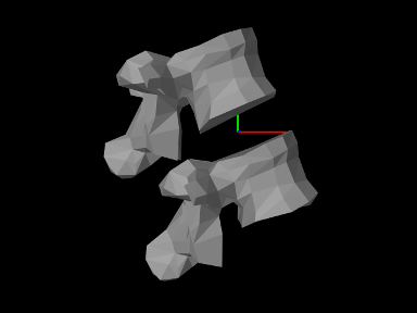
A simple model showing two simplified lumbar vertebrae, modeled as rigid bodies and connected by a frame spring, is defined in
artisynth.demos.tutorial.LumbarFrameSpring
The definition for the entire model class is shown here:
For convenience, the code to create and add each vertebrae is wrapped into the method addBone() defined at lines 27-32. This method takes two arguments: the MechModel to which the bone should be added, and the name of the bone. Surface meshes for the bones are located in .obj files located in the directory ../mech/geometry relative to the source directory for the model itself. PathFinder.getSourceRelativePath() is used to find a proper path to this directory (see Section 2.6) given the model class type (LumbarFrameSpring.class), and this is stored in the static string geometryDir. Within addBone(), the directory path and the bone name are used to create a path to the bone mesh itself, which is in turn used to create a PolygonalMesh (line 28). The mesh is then used in conjunction with a density to create a rigid body which is added to the MechModel (lines 29-30) and returned.
The build() method begins by creating and adding a MechModel, specifying a low value for gravity, and setting the rigid
body damping properties frameDamping and rotaryDamping (lines 37-41). (The damping parameters are needed
here because the frame spring itself is created with no damping.)
Rigid bodies representing the vertebrae lumbar1 and lumbar2 are then created by calling addBone() (lines 44-45),
lumbar1 is translated by setting the origin of its pose to
![]() , and lumbar2 is set to be fixed by making
it non-dynamic (line 47).
, and lumbar2 is set to be fixed by making
it non-dynamic (line 47).
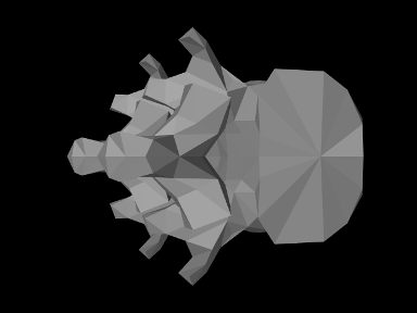
At this point in the construction, if the model were to be loaded, it
would appear as in Figure 3.34. To change
the viewpoint to that seen in Figure 3.33, we
rotate the entire model about the ![]() axis (line 50). This is done
using
transformGeometry(X), which transforms the geometry of an entire
model using a rigid or affine transform. This method is
described in more detail in Section 4.7.
axis (line 50). This is done
using
transformGeometry(X), which transforms the geometry of an entire
model using a rigid or affine transform. This method is
described in more detail in Section 4.7.
The frame spring is created and added at lines 54-59, using the methods described in Section 3.7.3, with frame D set to the (initial) pose of lumbar1.
Render properties are set starting at line 62. By default, a frame spring renders as a pair of red, green, blue coordinate axes showing frames C and D, along with a line connecting them. The line width and the color of the connecting line are controlled by the line render properties lineWidth and lineColor, while the length of the coordinate axes is controlled by the special frame spring property axisLength.
To run this example in ArtiSynth, select All demos > tutorial > LumbarFrameSpring from the Models menu. The model should load and initially appear as in Figure 3.33. Running the model (Section 1.5.3) will cause lumbar1 to fall slightly under gravity until the frame spring arrests the motion. To get a sense of the spring’s behavior, one can interactively apply forces to lumbar1 using the pull tool (see the section “Pull Manipulation” in the ArtiSynth User Interface Guide).
3.8 Other point-based forces
All ArtiSynth components which are capable of exerting forces, including the axial springs of Section 3.1 and the frame springs of Section 3.7, are subclasses of ForceComponent. Other force effector types include PointPlaneForce and PointMeshForce, described in this section.
3.8.1 Forces between points and planes or meshes
A PointPlaneForce component produces forces between a point
and a plane, based on the point’s signed distance ![]() from the plane.
Similarly, a PointMeshForce component produces forces
between one or more points and a closed polygonal mesh, based on the signed
distance
from the plane.
Similarly, a PointMeshForce component produces forces
between one or more points and a closed polygonal mesh, based on the signed
distance ![]() to the mesh. These components thus implement “soft” constraint
forces that bind points to either a plane or a mesh. If the component’s unilateral property is set to true, as described below, forces are
applied only when
to the mesh. These components thus implement “soft” constraint
forces that bind points to either a plane or a mesh. If the component’s unilateral property is set to true, as described below, forces are
applied only when ![]() . This allows the simulation of force-based contact
between points and planes or meshes.
. This allows the simulation of force-based contact
between points and planes or meshes.
PointPlaneForce and PointMeshForce can be used for particles, FEM nodes and point-based markers, all of which are subclasses of Point.
These force components result in a force ![]() acting on the point given by
acting on the point given by
where ![]() is the signed distance to the plane (or mesh),
is the signed distance to the plane (or mesh), ![]() is the plane
normal (or surface normal at the nearest mesh point),
is the plane
normal (or surface normal at the nearest mesh point), ![]() is a stiffness
force and
is a stiffness
force and ![]() is a damping constant. The stiffness force may be either linear
or quadratic, according to
is a damping constant. The stiffness force may be either linear
or quadratic, according to
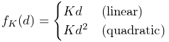 |
where ![]() is a stiffness constant and the choice of linear or quadratic is
controlled by the component’s forceType property.
is a stiffness constant and the choice of linear or quadratic is
controlled by the component’s forceType property.
If the component’s unilateral property is set to true, then the
computed force will be 0 whenever ![]() :
:
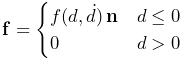 |
This allows plane and mesh force objects to implement “soft” collisions.
In the unilateral case, a quadratic force function provides smoother force transitions at
.
PointPlaneForce may be created with the following constructors:
| PointPlaneForce (Point p, Plane plane) |
Plane force component for point p |
| PointPlaneForce (Point p, Vector3d nrml, Point3d center) |
Plane is specified by its normal and center. |
Each of these creates a force component for a single point p, with the plane specified by either a Plane object or by its normal and center.
PointMeshForce may be created with the following constructors:
| PointMeshForce (MeshComponent mcomp) |
Mesh force for the mesh component mcomp. |
| PointMeshForce (String name, MeshComponent mcomp) |
Named mesh force for mesh mcomp. |
| PointMeshForce (String name, MeshComponent mcomp, double K, double D) |
Named mesh force with specified stiffness and damping. |
These create PointMeshForce for a mesh contained within a MeshComponent (Section 3.3). The mesh must be a polygonal mesh composed of triangles.
The points associated with a PointMeshForce are added after creation. The following methods are used to manage the point set:
| void addPoint (Point p) |
Adds point p. |
| boolean removePoint (Point p) |
Removes point p. |
| int numPoints() |
Returns the number of points. |
| Point getPoint (int idx) |
Returns the idx-th point. |
| void clearAllPoints() |
Removes all points. |
PointPlaneForce and PointMeshForce export a variety of properties that control their force behavior and appearance:
-
•
stiffness: A double value giving the stiffness constant
 .
Default value 1.0.
.
Default value 1.0. -
•
damping: A double value giving the damping constant
 .
Default value 0.0.
.
Default value 0.0. -
•
forceType: A value of type PointPlaneForce.ForceType or PointMeshForce.ForceType which describes the stiffness force, with the options being LINEAR and QUADRATIC. Default value LINEAR.
-
•
unilateral: A boolean value, which if true means that no force will be generated for
 . Default value false for
PointPlaneForce and true for PointMeshForce.
. Default value false for
PointPlaneForce and true for PointMeshForce. -
•
enabled: A boolean value, which if false disables the component so that it will generate no force. Default value true.
-
•
planeSize: For PointPlaneForce only, a double value that gives the size of the plane for rendering purposes only. Default value 1.0.
The forces acting on each point can also be rendered in the viewer by setting the following additional properties:
-
•
drawForces: A boolean value, which if true causes the force on each point to be rendered using a line segment drawn from the point in the direction of the force. The length of each line segment is given by the force magnitude times the value of the forceLenScale property. Other render properties are controlled by the component’s generic line rendering properties.
-
•
forceLenScale: A double value, which if drawForces is true, is multiplied by the magnitude of each point force to determine the length of the rendered line segment.
These properties can be set either interactively in the GUI, or in code using their accessor methods.
3.8.2 Example: point plane forces
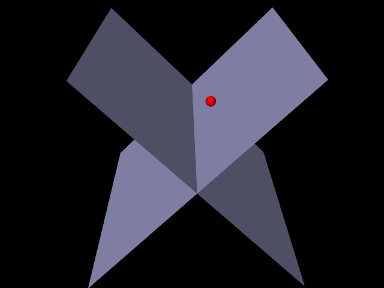
An example using PointPlaneForce is given by
artisynth.demos.tutorial.PointPlaneForces
which implements soft collision between a particle and two planes. The build() method is shown below:
A MechModel is created in the usual way (lines 2-3), followed by a
particle (lines 6-7). Then two PointPlaneForces are created to act on
this particle (lines 10-24), each centered on the origin, with plane normals of
![]() and
and ![]() , respectively. The forces are unilateral and
linear (the default), with a stiffness of 1000. Each plane’s size is set to 5;
this is for rendering purposes only, as the planes have infinite extent for
purposes of force calculation. Lastly, rendering properties are set (lines
27-28) to make the particle appear as a red sphere and the planes blue-gray.
, respectively. The forces are unilateral and
linear (the default), with a stiffness of 1000. Each plane’s size is set to 5;
this is for rendering purposes only, as the planes have infinite extent for
purposes of force calculation. Lastly, rendering properties are set (lines
27-28) to make the particle appear as a red sphere and the planes blue-gray.
To run this example in ArtiSynth, select All demos > tutorial > PointPlaneForces from the Models menu. When run, the particle will drop and bounce off the planes (Figure 3.35), finally coming to rest along the line where they intersect.
This model does not include damping, and so damping effects are due entirely to the default implicit integrator ConstrainedBackwardEuler. If the integrator is changed to an explicit one, using a directive such as
then the ball will continue to bounce during the simulation.
3.8.3 Example: point mesh forces
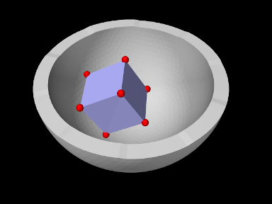
An example using PointMeshForce is given by
artisynth.demos.tutorial.PointMeshForces
which implements soft collision between a rigid cube and a bowl-shaped mesh, using a PointMeshForce to create force between the mesh and markers at the cube corners. The build() method is shown below:
A MechModel is created (lines 3-5), with inertialDamping set to 1.0 to help reduce oscillations as the cube bounces off the bowl. The cube itself is created as a RigidBody and positioned so as to fall into the bowl under gravity (lines 8-12). A frame marker is placed at each of the cube’s corners, using the (local) positions of its surface mesh vertices to determine the marker locations (lines 13-18); these markers will act as the collision points.
The bowl is constructed as a FixedMeshBody containing a mesh
read from the folder "data/" located beneath the source folder of the
model (lines 8-12). A PointMeshForce is then allocated for the bowl
(lines 28-34), with unilateral behavior (the default) and a quadratic stiffness
force with ![]() and
and ![]() . Each marker point is added to it to
enforce the collision. Lastly, rendering properties are set (lines 38-40) to
set the colors for the cube and bowl and make the markers appear as a red
spheres.
. Each marker point is added to it to
enforce the collision. Lastly, rendering properties are set (lines 38-40) to
set the colors for the cube and bowl and make the markers appear as a red
spheres.
To run this example in ArtiSynth, select All demos > tutorial > PointMeshForces from the Models menu. When run, the cube will drop into the bowl and bounce around (Figure 3.36).
Because of the discrete nature of the simulation, force-based collision handling is subject to the same time step limitations as constraint-based collisions (Section 8.9). In particular, insufficiently small time steps, or too small a stiffness, may cause objects to pass through each other. Insufficient damping may also result in excessive bouncing.
3.9 Attachments
ArtiSynth provides the ability to rigidly attach dynamic components to other dynamic components, allowing different parts of a model to be connected together. Attachments are made by adding to a MechModel special attachment components that manage the attachment physics as described briefly in Section 1.2.3.
3.9.1 Point attachments
Point attachments allow particles and other point-based components to be attached to other, more complex components, such as frames, rigid bodies, or finite element models (Section 6.4). Point attachments are implemented by creating attachment components that are instances of PointAttachment. Modeling applications do not generally handle the attachment components directly, but instead create them implicitly using the following MechModel method:
This attaches a point p1 to any component which implements the interface PointAttachable, indicating that it is capable of creating an attachment to a point. Components that implement PointAttachable currently include rigid bodies, particles, and finite element models. The attachment is created based on the current position of the point and component in question. For attaching a point to a rigid body, another method may be used:
This attaches p1 to body at the point loc specified in body coordinates. Finite element attachments are discussed in Section 6.4.
3.9.2 Example: model with particle attachments
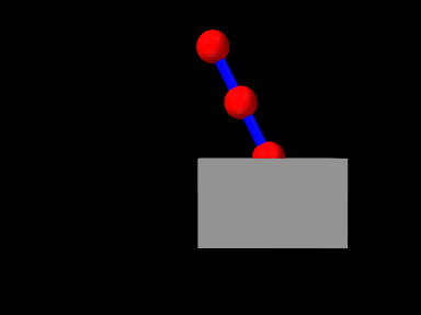
A model illustrating particle-particle and particle-rigid body attachments is defined in
artisynth.demos.tutorial.ParticleAttachment
and most of the code is shown here:
The code is very similar to ParticleSpring and RigidBodySpring described in Sections 3.1.5 and 3.2.2, except that two convenience methods, addParticle() and addSpring(), are defined at lines 1-15 to create particles and spring and add them to a MechModel. These are used in the build() method to create four particles and two springs (lines 24-29), along with a rigid body box (lines 31-34). As with the other examples, particle p1 is set to be non-dynamic (line 36) in order to fix it in place and provide a ground.
The attachments are added at lines 39-40, with p2 attached to
p3 and p4 connected to the box at the location ![]() in box coordinates.
in box coordinates.
Finally, render properties are set starting at line 43. In this example, point and line render properties are set for the entire MechModel instead of individual components. Since render properties are inherited, this will implicitly set the specified render properties in all subcomponents for which these properties are not explicitly set (either locally or in an intermediate ancestor).
3.9.3 Frame attachments
Frame attachments allow rigid bodies and other frame-based components to be attached to other components, including frames, rigid bodies, or finite element models (Section 6.6). Frame attachments are implemented by creating attachment components that are instances of FrameAttachment.
As with point attachments, modeling applications do not generally handle frame attachment components directly, but instead create and add them implicitly using the following MechModel methods:
These attach frame to any component which implements the interface FrameAttachable, indicating that it is capable of creating an attachment to a frame. Components that implement FrameAttachable currently include frames, rigid bodies, and finite element models. For the first method, the attachment is created based on the current position of the frame and component in question. For the second method, the attachment is created so that the initial pose of the frame (in world coordinates) is described by TFW.
Once a frame is attached, it will be in the attached state, as described in Section 1.2.4. Frame attachments can be removed by calling
While it is possible to create composite rigid bodies using FrameAttachments, this is much less computationally efficient (and less accurate) than creating a single rigid body through mesh merging or similar techniques.
3.9.4 Example: model with frame attachments
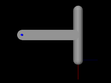
A model illustrating rigidBody-rigidBody and frame-rigidBody attachments is defined in
artisynth.demos.tutorial.FrameBodyAttachment
Most of the code is identical to that for RigidBodyJoint as described in Section 3.4.6, except that the joint is further to the left and connects bodyB to ground, rather than to bodyA, and the initial pose of bodyA is changed so that it is aligned vertically. bodyA is then connected to bodyB, and an auxiliary frame is created and attached to bodyA, using code at the end of the build() method as shown here:
To run this example in ArtiSynth, select All demos > tutorial > FrameBodyAttachment from the Models menu. The model should load and initially appear as in Figure 3.37. The frame attached to bodyA is visible in the lower right corner. Running the model (Section 1.5.3) will cause both bodies to fall and swing about the joint under gravity.
3.10 Attached frames
In the same sense that a Marker is a point attached to another dynamic component, an AttachedFrame is a coordinate frame attached to a dynamic component.
3.10.1 Frame attached frames
A FrameAttachedFrame is an AttachedFrame that is
rigidly connected to a master Frame (which includes
RigidBody as a subclass), in the same way that a FrameMarker is a point attached to a Frame. Once attached, the FrameAttachedFrame moves rigidly with its master frame. The relative pose of
the attached frame with respect to its master is described by the transform
![]() , referred to in the code examples as TFM.
, referred to in the code examples as TFM.
FrameAttachedFrame objects can be created using a variety of constructors, including
| FrameAttachedFrame () | |
| FrameAttachedFrame (String name) | |
| FrameAttachedFrame (RigidTransform3d TFW) | |
| FrameAttachedFrame (Frame frame, RigidTransform3d TFW) |
where FrameAttachedFrame() creates a default frame with no master
assigned, FrameAttachedFrame(name) adds a name, and FrameAttachedFrame(TFW) initializes the world pose to TFW. The
last constructor also attaches the frame to frame, with ![]() computed from the two frames’ current world poses. After construction,
the master frame can be set and queried using
computed from the two frames’ current world poses. After construction,
the master frame can be set and queried using
| void setFrame (Frame frame) | |
| Frame getFrame () |
where setFrame(frame) computes ![]() from the attached frame’s
current world pose and the master’s world pose. The transform
from the attached frame’s
current world pose and the master’s world pose. The transform ![]() and
the world pose
and
the world pose ![]() can also be set and queried directly:
can also be set and queried directly:
| RigidTransform3d getTFM () |
Returns |
| void setTFM (RigidTransform3d TFM) |
Sets |
| void setTFW (RigidTransform3d TFW) |
Sets |
Note there is no need for a getTFW() method because that is the same as
the frame’s getPose() method, whereas setTFW() differs from setPose(TFW) because the former updates ![]() to accommodate the new value
of
to accommodate the new value
of ![]() , while the latter does not and so the frame will revert back to
the pose imparted by the master.
, while the latter does not and so the frame will revert back to
the pose imparted by the master.
Created FrameAttachedFrame objects must be added to the MechModel. One way to do this is to add them to the model’s frames container, which is managed using the MechModel methods:
| void addFrame (Frame frame) |
Adds frame frame to the container. |
| boolean removeFrame (Frame frame) |
Removes frame frame from the container. |
| void clearFrames() |
Removes all frames. |
| RenderableComponentList<Frame> frames() |
Returns the frames container. |
FrameAttachedFrame objects can be added directly to a Frame component, which maintains an attachedFrames container as a subcomponent. Attached frames can be added to this list using
| void addAttachedFrame (FrameAttachedFrame frm) |
Adds an existing FrameAttachedFrame to a frame, setting its master to frame if necessary. |
| FrameAttachedFrame addAttachedFrame ( RigidTransform3d TFM) |
Creates a FrameAttachedFrame at pose |
| FrameAttachedFrame addAttachedFrameWorld ( RigidTransform3d TFW) |
Creates a FrameAttachedFrame at pose |
The attachedFrames container can be accessed and frames removed using
| RenderableComponentList<FrameAttachedFrame> getAttachedFrames () |
Returns the frame’s attachedFrames container. |
| boolean removeAttachedFrame ( FrameAttachedFrame frm) |
Removes frm from the container; returns true if it was present. |
| void clearAttachedFrames () |
Removes all frames from the container. |
3.10.2 Example: attached frames for a rigid body
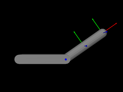
A model demonstrating the attachment of frames to a rigid body is defined in
artisynth.demos.tutorial.RigidBodyAttachedFrames
This subclasses RigidBodyJoint (Section 3.4.6) and
extends its build() method to add two FrameAttachedFrames to bodyA, one specified via ![]() and one via the world pose
and one via the world pose ![]() :
:
The first attached frame, frameAtTip, is created using addAttachedFrame(TFM), with ![]() placing it at the tip of bodyA
along its local
placing it at the tip of bodyA
along its local ![]() -axis. The second, frameAtCenter, is created using
addAttachedFrameWorld(TFW), with its world pose set to match the
current pose of bodyA, so it sits at the body’s origin. Both frames
are rendered as solid arrow triads (AxisDrawStyle.ARROW).
-axis. The second, frameAtCenter, is created using
addAttachedFrameWorld(TFW), with its world pose set to match the
current pose of bodyA, so it sits at the body’s origin. Both frames
are rendered as solid arrow triads (AxisDrawStyle.ARROW).
To run this example in ArtiSynth, select All demos > tutorial > RigidBodyAttachedFrames from the Models menu. The model should load and initially appear as in Figure 3.39. Running the model will cause bodyA to swing under gravity, with both attached frames moving rigidly with it.
Chapter 4 Mechanical Models II
This section provides additional material on building basic multibody-type mechanical models.
4.1 Simulation control properties
4.1.1 Simulation step size
One of the most important properties is maxStepSize. By default, simulation proceeds using the maxStepSize value defined for the root model. A MechModel (or any other type of Model) contained in the root model’s models list may also request a smaller step size by specifying a smaller value for its own maxStepSize property. For all models, the maxStepSize may be set and queried using
4.1.2 Integrator
Another important simulation property is integrator in MechModel, which determines the type of integrator used for the physics simulation. The value type of this property is the enumerated type MechSystemSolver.Integrator, for which the following values are currently defined:
- ForwardEuler
-
First order forward Euler integrator. Unstable for stiff systems.
- SymplecticEuler
-
First order symplectic Euler integrator, more energy conserving than forward Euler. Unstable for stiff systems.
- RungeKutta4
-
Fourth order Runge-Kutta integrator, quite accurate but also unstable for stiff systems.
- ConstrainedBackwardEuler
-
First order backward Euler integrator. Generally stable for stiff systems.
- Trapezoidal
-
Second order trapezoidal integrator. Generally stable for stiff systems, but slightly less so thanConstrainedBackwardEuler.
The term “Unstable for stiff systems” means that the integrator is likely to go unstable in the presence of “stiff” systems, which typically include systems containing finite element models, unless the simulation step size is set to an extremely small value. The default value for integrator is ConstrainedBackwardEuler.
Stiff systems tend to arise in models containing interconnected deformable elements, for which the step size should not exceed the propagation time across the smallest element, an effect known as the Courant-Friedrichs-Lewy (CFL) condition. Larger stiffness and damping values decrease the propagation time and hence the allowable step size.
4.1.3 Position stabilization
Another MechModel simulation property is stabilization, which controls the stabilization method used to correct drift from position constraints and correct interpenetrations due to collisions (Chapter 8). The value type of this property value is the enumerated type MechSystemSolver.PosStabilization, which presently has two values:
- GlobalMass
-
Uses only a diagonal mass matrix for the MLCP that is solved to determine the position corrections. This is the default method.
- GlobalStiffness
-
Uses a stiffness-corrected mass matrix for the MLCP that is solved to determine the position corrections. Slower than GlobalMass, but more likely to produce stable results, particularly for problems involving FEM collisions.
4.2 Units
ArtiSynth is primarily “unitless”, in the sense that it does not
define default units for the fundamental physical quantities of time,
length, and mass. Although time is
generally understood to be in seconds, and often declared as such in
method arguments and return values, there is no hard requirement that
it be interpreted as seconds. There are no assumptions at all
regarding length and mass. Some components may have default parameter
values that reflect a particular choice of units, such as MechModel’s default gravity value of ![]() , which is
associated with the MKS system, but these values can always be
overridden by the application.
, which is
associated with the MKS system, but these values can always be
overridden by the application.
Nevertheless, it is important, and up to the application developer to
ensure, that units be consistent. For example, if one decides to
switch length units from meters to centimeters (a common choice),
then all units involving length will have to be scaled appropriately.
For example, density, whose fundamental units are ![]() , where
, where ![]() is mass and
is mass and
![]() is distance, needs to be scaled by
is distance, needs to be scaled by ![]() , or
, or ![]() , when
converting from meters to centimeters.
, when
converting from meters to centimeters.
Table 4.1 lists a number of common physical quantities used in ArtiSynth, along with their associated fundamental units.
| unit | fundamental units | |
|---|---|---|
| time | ||
| distance | ||
| mass | ||
| velocity | ||
| acceleration | ||
| force | ||
| work/energy | ||
| torque | same as energy (somewhat counter intuitive) | |
| angular velocity | ||
| angular acceleration | ||
| rotational inertia | ||
| pressure | ||
| Young’s modulus | ||
| Poisson’s ratio | 1 | no units; it is a ratio |
| density | ||
| linear stiffness | ||
| linear damping | ||
| rotary stiffness | same as torque | |
| rotary damping | ||
| mass damping | used in FemModel | |
| stiffness damping | used in FemModel |
4.2.1 Scaling units
For convenience, many ArtiSynth components, including MechModel, implement the interface ScalableUnits, which provides the following methods for scaling mass and distance units:
A call to one of these methods should cause all physical quantities within the component (and its descendants) to be scaled as required by the fundamental unit relationships as shown in Table 4.1.
Converting a MechModel from meters to centimeters can therefore be easily done by calling
As an example, adding the following code to the end of the build() method in RigidBodySpring (Section 3.2.2)
will scale the distance units by 100 and print the values of various quantities before and after scaling. The resulting output is:
It is important not to confuse scaling units with scaling the actual geometry or mass. Scaling units should change all physical quantities so that the simulated behavior of the model remains unchanged. If the distance-scaled version of RigidBodySpring shown above is run, it should behave exactly the same as the non-scaled version.
4.3 Render properties
All ArtiSynth components that are renderable maintain a property renderProps, which stores a RenderProps object that contains a number of subproperties used to control an object’s rendered appearance.
In code, the renderProps property for an object can be set or queried using the methods
Render properties can also be set in the GUI by selecting one or more components and then choosing Set render props ... in the right-click context menu. More details on setting render properties through the GUI can be found in the section “Render properties” in the ArtiSynth User Interface Guide.
For many components, the default value of renderProps is null; i.e., no RenderProps object is assigned by default and render properties are instead inherited from ancestor components further up the hierarchy. The reason for this is because RenderProps objects are fairly large (many kilobytes), and so assigning a unique one to every component could consume too much memory. Even when a RenderProps object is assigned, most of its properties are inherited by default, and so only those properties which are explicitly set will differ from those specified in ancestor components.
4.3.1 Render property taxonomy
In general, the properties in RenderProps are used to control the color, size, and style of the three primary rendering primitives: faces, lines, and points. Table 4.2 contains a complete list. Values for the shading, faceStyle, lineStyle and pointStyle properties are defined using the following enumerated types: Renderer.Shading, Renderer.FaceStyle, Renderer.PointStyle, and Renderer.LineStyle. Colors are specified using java.awt.Color.
| property | purpose | usual default value |
| visible | whether or not the component is visible | true |
| alpha | transparency for diffuse colors (range 0 to 1) | 1 (opaque) |
| shading | shading style: (FLAT, SMOOTH, METAL, NONE) | FLAT |
| shininess | shininess parameter (range 0 to 128) | 32 |
| specular | specular color components | null |
| faceStyle | which polygonal faces are drawn (FRONT, BACK, FRONT_AND_BACK, NONE) | FRONT |
| faceColor | diffuse color for drawing faces | GRAY |
| backColor | diffuse color used for the backs of faces. If null, faceColor is used. | null |
| drawEdges | hint that polygon edges should be drawn explicitly | false |
| colorMap | color mapping properties (see Section 4.3.3) | null |
| normalMap | normal mapping properties (see Section 4.3.3) | null |
| bumpMap | bump mapping properties (see Section 4.3.3) | null |
| edgeColor | diffuse color for edges | null |
| edgeWidth | edge width in pixels | 1 |
| lineStyle: | how lines are drawn (CYLINDER, LINE, or SPINDLE) | LINE |
| lineColor | diffuse color for lines | GRAY |
| lineWidth | width in pixels when LINE style is selected | 1 |
| lineRadius | radius when CYLINDER or SPINDLE style is selected | 1 |
| pointStyle | how points are drawn (SPHERE or POINT) | POINT |
| pointColor | diffuse color for points | GRAY |
| pointSize | point size in pixels when POINT style is selected | 1 |
| pointRadius | sphere radius when SPHERE style is selected | 1 |
To increase and improve their visibility, both the line and point primitives are associated with styles (CYLINDER, SPINDLE, and SPHERE) that allow them to be rendered using 3D surface geometry.
Exactly how a component interprets its render properties is up to the component (and more specifically, up to the rendering method for that component). Not all render properties are relevant to all components, particularly if the rendering does not use all of the rendering primitives. For example, Particle components use only the point primitives and AxialSpring components use only the line primitives. For this reason, some components use subclasses of RenderProps, such as PointRenderProps and LineRenderProps, that expose only a subset of the available render properties. All renderable components provide the method createRenderProps() that will create and return a RenderProps object suitable for that component.
4.3.2 Setting render properties
When setting render properties, it is important to note that the value returned by getRenderProps() should be treated as read-only and should not be used to set property values. For example, applications should not do the following:
This can cause problems for two reasons. First, getRenderProps() will return null if the object does not currently have a RenderProps object. Second, because RenderProps objects are large, ArtiSynth may try to share them between components, and so by setting them for one component, the application may inadvertently set them for other components as well.
Instead, RenderProps provides a static method for each property that can be used to set that property’s value for a specific component. For example, the correct way to set pointColor is
One can also set render properties by calling setRenderProps() with a predefined RenderProps object as an argument. This is useful for setting a large number of properties at once:
For setting each of the color properties within RenderProps, one can use either Color objects or float[] arrays of length 3 giving the RGB values. Specifically, there are methods of the form
as well as the static methods
where XXX corresponds to Point, Line, Face, Edge, and Back. For Edge and Back, both color and rgb can be given as null to clear the indicated color. For the specular color, the associated methods are
Note that even though components may use a subclass of RenderProps internally, one can always use the base RenderProps class to set values; properties which are not relevant to the component will simply be ignored.
Finally, as mentioned above, render properties are inherited. Values set high in the component hierarchy will be inherited by descendant components, unless those descendants (or intermediate components) explicitly set overriding values. For example, a MechModel maintains its own RenderProps (and which is never null). Setting its pointColor property to RED will cause all point-related components within that MechModel to be rendered as red except for components that set their pointColor to a different value.
There are typically three levels in a MechModel component hierarchy at which render properties can be set:
-
•
The MechModel itself;
-
•
Lists containing components;
-
•
Individual components.
For example, consider the following code:
Setting the MechModel render property pointColor to BLUE will cause all point-related items to be rendered blue by default. Setting the pointColor render property for the particle list (returned by mech.particles()) will override this and cause all particles in the list to be rendered green by default. Lastly, setting pointColor for p3 will cause it to be rendered as red.
4.3.3 Texture mapping
Render properties can also be set to apply texture mapping to objects containing polygonal meshes in which texture coordinates have been set. Support is provided for color, normal and bump mapping, although normal and bump mapping are only available under the OpenGL 3 version of the ArtiSynth renderer.
Texture mapping is controlled through the colorMap, normalMap, and bumpMap properties of RenderProps. These are composite properties with a default value of null, but applications can set them to instances of ColorMapProps, NormalMapProps, and BumpMapProps, respectively, to provide the source images and parameters for the associated mapping. The two most important properties exported by all of these MapProps objects are:
- enabled
-
A boolean indicating whether or not the mapping is enabled.
- fileName
-
A string giving the file name of the supporting source image.
NormalMapProps and BumpMapProps also export scaling,
which scales the x-y components of the normal map or the depth of the
bump map. Other exported properties control mixing with underlying
colors, and how texture coordinates are both filtered and managed when
they fall outside the canonical range ![]() . Full details on
texture mapping and its support by the ArtiSynth renderer are given in
the “Rendering” section of the
Maspack Reference Manual.
. Full details on
texture mapping and its support by the ArtiSynth renderer are given in
the “Rendering” section of the
Maspack Reference Manual.
To set up a texture map, one creates an instance of the appropriate MapProps object and uses this to set either the colorMap, normalMap, or bumpMap property of RenderProps. For a specific renderable, the map properties can be set using the static methods
When initializing the MapProps object, it is often sufficient to just set enabled to true and fileName to the full path name of the source image. Normal and bump maps also often require adjustment of their scaling properties. The following static methods are available for setting the enabled and fileName subproperties within a renderable:
Normal and bump mapping only work under the OpenGL 3 version of the ArtiSynth viewer, and also do not work if the shading property of RenderProps is set to NONE or FLAT.
Texture mapping properties can be set within ancestor nodes of the component hierarchy, to allow file names and other parameters to be propagated throughout the hierarchy. However, when this is done, it is still necessary to ensure that the corresponding mapping properties for the relevant descendants are non-null. That’s because mapping properties themselves are not inherited; only their subproperties are. If a mapping property for any given object is null, the associated mapping will be disabled. A non-null mapping property for an object will be created automatically by calling one of the setXXXEnabled() methods listed above. So when setting up ancestor-controlled mapping, one may use a construction like this:
RenderProps.setColorMap (ancestor, tprops); RenderProps.setColorMapEnabled (descendant0, true); RenderProps.setColorMapEnabled (descendant1, true);Then colorMap subproperties set within ancestor will be inherited by descendant0 and descendant1.
As indicated above, texture mapping will only be applied to components containing rendered polygonal meshes for which appropriate texture coordinates have been set. Determining such texture coordinates that produce appropriate results for a given source image is often non-trivial; this so-called “u-v mapping problem” is difficult in general and is highly dependent on the mesh geometry. ArtiSynth users can handle the problem of assigning texture coordinates in several ways:
-
•
Use meshes which already have appropriate texture coordinates defined for a given source image. This generally means that mesh is specified by a file that contains the required texture coordinates. The mesh should then be read from this file (Section 2.5.5) and then used in the construction of the relevant components. For example, the application can read in a mesh containing texture coordinates and then use it to create a RigidBody via the method RigidBody.createFromMesh().
-
•
Use a simple mesh object with predefined texture coordinates. The class MeshFactory provides the methods
PolygonalMesh createRectangle (width, height, xdivs, ydivs, addTextureCoords);PolygonalMesh createSphere (radius, nslices, nlevels, addTextureCoords)which create rectangular and spherical meshes, along with canonical texture coordinates if addTextureCoords is true. Coordinates generated by createSphere() are defined so that
 and
and  map to the spherical coordinates
  (at
the south pole) and
(at
the south pole) and  (at the north pole). Source images can
be relatively easy to find for objects with canonical coordinates.
(at the north pole). Source images can
be relatively easy to find for objects with canonical coordinates. -
•
Compute custom texture coordinates and set them within the mesh using setTextureCoords().
An example where texture mapping is applied to spherical meshes to make them appear like tennis balls is defined in
artisynth.demos.tutorial.SphericalTextureMapping
and listing for this is given below:
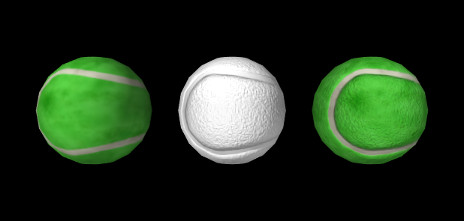
The build() method uses the internal method createBall() to generate three rigid bodies, each defined using a spherical mesh that has been created with MeshFactory.createSphere() with addTextureCoords set to true. The remainder of the build() method sets up the render properties and the texture mappings. Two texture mappings are defined: a color mapping and bump mapping, based on the images TennisBallColorMap.jpg and TennisBallBumpMap.jpg (Figure 4.2), both located in the subdirectory data relative to the demo source file. PathFinder.expand() is used to determine the full data folder name relative to the source directory. For the bump map, it is important to set the scaling property to adjust the depth amplitude to relative to the sphere radius.
 |
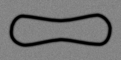 |
Color mapping is applied to balls 0 and 2, and bump mapping to balls 1 and 2. This is done by setting color map and/or bump map render properties in the components holding the actual meshes, which in this case is the mesh components for the balls’ surfaces meshes, obtained using getSurfaceMeshComp(). As mentioned above, it is also possible to set these render properties in an ancestor component, and that is done here by setting the colorMap render property of the MechModel, but then it is also necessary to enable color mapping within the individual mesh components, using RenderProps.setColorMapEnabled().
To run this example in ArtiSynth, select All demos > tutorial > SphericalTextureMapping from the Models menu. The model should load and initially appear as in Figure 4.1. Note that if ArtiSynth is run with the legacy OpenGL 2 viewer (command line option -GLVersion 2), bump mapping will not be supported and will not appear.
4.4 Custom rendering
It is often useful to add custom rendering to an application. For example, one may wish to render forces acting on bodies, or marker positions that are not otherwise assigned to a component. Custom rendering is relatively easy to do, as described in this section.
4.4.1 Component render() methods
All renderable ArtiSynth components implement the IsRenderable interface, which contains the methods prerender() and render(). As its name implies, prerender() is called prior to rendering and is discussed in Section 4.4.4. The render() method, discussed here, performs the actual rendering. It has the signature
where the Renderer supplies a large set of methods for performing the rendering, and flags is described in the API documentation. The methods supplied by the renderer include ones for drawing simple primitives such as points, lines, and triangles; simple 3D shapes such as cubes, cones, cylinders and spheres; and text components.
A full description of the Renderer can be obtained by checking its API documentation and also by consulting the “Rendering” section of the Maspack Reference Manual.
A small sampling of the methods supplied by a Renderer include:
For example, the render() implementation below renders three spheres connected by pixel-based lines, as show in Figure 4.3 (left):
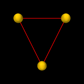
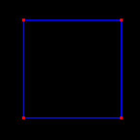
|
A Renderer also contains draw mode methods to implement the drawing of points, lines and triangles in a manner similar to the immediate mode of legacy OpenGL,
where drawMode is an instance of Renderer.DrawMode and includes points, lines, line strips and loops, triangles, and triangle strips and fans. The draw mode methods include:
| void beginDraw(DrawMode mode) |
Begin a draw mode sequence. |
| void addVertex(Vector3d vtx) |
Add a vertex to the object being drawn. |
| void setNormal(Vector3d nrm) |
Sets the current vertex normal for the object being drawn. |
| void endDraw() |
Finish a draw mode sequence. |
The render() implementation below uses draw mode to render the image shown in Figure 4.3, right:
Finally, a Renderer contains methods for the rendering of render objects, which are collections of vertex, normal and color information that can be rendered quickly; it may be more efficient to use render objects for complex rendering involving large numbers of primitives. Full details on this, and other features of the rendering interface, are given in the “Rendering” section of the Maspack Reference Manual.
4.4.2 Implementing custom rendering
There are two easy ways to add custom rendering to a model:
-
1.
Override the root model’s render() method;
-
2.
Define a custom rendering component, with its own render() method, and add it to the model. This approach is more modular and makes it easier to reuse the rendering between models.
To override the root model render method, one simply adds the following declaration to the model’s definition:
A call to super.render() is recommended to ensure that any rendering done by the model’s base class will still occur. Subsequent statements should then use the renderer object to perform whatever rendering is required, using methods such as described in Section 4.4.1 or in the “Rendering” section of the Maspack Reference Manual.
To create a custom rendering component, one can simply declare a subclass of RenderableComponentBase with a custom render() method:
There is no need to call super.render() since RenderableComponentBase does not provide an implementation of render(). It does, however, provide default implementations of everything else required by the Renderable interface. This includes exporting render properties via the composite property renderProps, which the render() method may use to control the rendering appearance in a manner consistent with Section 4.3.2. It also includes an implementation of prerender() which by default does nothing. As discussed more in Section 4.4.4, this is often acceptable unless:
-
1.
rendering will be adversely affected by quantities being updated asynchronously within the simulation;
-
2.
the component contains subcomponents that also need to be rendered.
Once a custom rendering component has been defined, it can be created and added to the model within the build() method:
In this example, the component is added to the MechModel’s subcomponent list renderables, which ensures that it will be found by the rendering code. Methods for managing this list include:
| void addRenderable(Renderable r) |
Adds a renderable to the model. |
| boolean removeRenderable(Renderable r) |
Removes a renderable from the model. |
| void clearRenderables() |
Removes all renderables from the model. |
| ComponentListView<RenderableComponent> renderables() |
Returns the list of all renderables. |
4.4.3 Example: rendering body forces
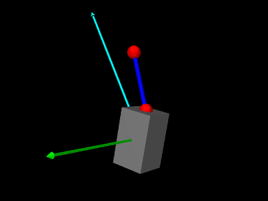
The application model
artisynth.demos.tutorial.BodyForceRendering
gives an example of custom rendering to draw the force and moment vectors acting on a rigid body as cyan and green arrows, respectively. The model extends RigidBodySpring (Section 3.2.2), defines a custom renderable class named ForceRenderer, and then uses this to render the forces on the box in the original model. The code, with the include files omitted, is listed below:
The force renderer is defined at lines (4-34). For attributes, it contains a reference to the rigid body, plus scale factors for rendering the force and moment. Within the render() method (lines 16-33), the force and moment vectors are drawn as cyan and green arrows, starting at the current body position, and scaled by their respective factors. This scaling is needed to ensure the arrows have a size appropriate to the viewer, and separate scale factors are needed because the force and moment vectors have different units. The arrow radii are given by the renderer’s lineRadius render property (lines 22 and 30).
The build() method starts by calling the super class build() method to create the original model (line 36), and then uses findComponent() to retrieve its MechModel, within which the “box” rigid body is located (lines 40-41). A ForceRenderer is then created for this body, with force and moment scale factors of 0.1 and 0.5, and added to the MechModel (lines 44-45). The renderer’s lineRadius render property is then set to 0.01 (line 48).
To run this example in ArtiSynth, select All demos > tutorial > BodyForceRenderer from the Models menu. When run, the model should appear as in Figure 4.4, showing the force and moment vectors acting on the box.
4.4.4 The prerender() method
Component render() methods are called within ArtiSynth’s graphics thread, and so are called asynchronously with respect to the simulation thread(s). This means that the simulation may be updating component attributes, such as positions or forces, at the same time they are being accessed within render(), leading to inconsistent results in the viewer. While these inconsistencies may not be significant, particularly if the attributes are changing slowly between time steps, some applications may wish to avoid them. For this, renderable components also implement a prerender() method, with the signature
that is called in synchronization with the simulation prior to rendering. Its purpose is to:
-
•
Make copies of simulation-varying attributes so that they can be used without conflict in the render() method;
-
•
Identify to the system any additional subcomponents that also need to be rendered.
The first task is usually accomplished by copying simulation-varying attributes into cache variables stored within the component itself. For example, if a component is responsible for rendering the forces of a rigid body (as per Section 4.4.3), it may wish to make a local copy of these forces within prerender:
The second task, identifying renderable subcomponents, is accomplished using the addIfVisible() and addIfVisibleAll() methods of the RenderList argument, as in the following examples:
It should be noted that some ArtiSynth components already support cached copies of attributes that can be used for rendering. In particular, Point (whose subclasses include Particle and FemNode3d) uses prerender() to cache its position as an array of float[] which can be obtained using getRenderCoords(), and Frame (whose subclasses include RigidBody) caches its pose as a RigidTransform3d that can be obtained with getRenderFrame().
4.5 Point-to-point muscles, tendons and ligaments
Point-to-point muscles are a simple type of component in biomechanical models that provide muscle-activated forces acting along a line between two points. ArtiSynth provides this through Muscle, which is a subclass of AxialSpring that generates an active muscle force in response to its excitation property. The excitation property can be set and queried using the methods
As with AxialSprings, Muscle components use subclasses of
AxialMaterial to compute the
applied force ![]() in response to the muscle’s length
in response to the muscle’s length
![]() , length velocity
, length velocity ![]() , and excitation signal
, and excitation signal ![]() , which is
assumed to lie in the interval
, which is
assumed to lie in the interval ![]() . Special muscle
subclasses of AxialMaterial exist that compute forces that vary
in response to the excitation. As with other axial materials, this is
done by the material’s computeF() method, first described in
Section 3.1.7:
. Special muscle
subclasses of AxialMaterial exist that compute forces that vary
in response to the excitation. As with other axial materials, this is
done by the material’s computeF() method, first described in
Section 3.1.7:
Usually the force is the sum of a passive component plus an active component that arises in response to the excitation signal.
Once a muscle material is created, it can be assigned to a muscle or queried using Muscle methods
Muscle materials can also be assigned to axial springs, although the resulting force will always be computed with 0 excitation.
4.5.1 Simple muscle materials
A number of simple muscle materials are described below. All compute
force as a function of ![]() and
and ![]() , with an optional damping force
that is proportional to
, with an optional damping force
that is proportional to ![]() . More complex Hill-type muscles, with
force velocity curves, pennation angle, and a tendon component in
series, are also available and described in
Section 4.5.3.
. More complex Hill-type muscles, with
force velocity curves, pennation angle, and a tendon component in
series, are also available and described in
Section 4.5.3.
For historical reasons, the materials ConstantAxialMuscle, LinearAxialMuscle and PeckAxialMuscle, described below, contain a property called forceScaling that uniformly scales the computed force. This property is now deprecated, and should therefore have a value of 1. However, creating these materials with constructors not indicated in the documentation below will cause forceScaling to be set to a default value of 1000, thus requiring that the maximum force and damping values be correspondingly reduced.
4.5.1.1 SimpleAxialMuscle
SimpleAxialMuscle is the default AxialMaterial for Muscle, and is essentially an activated version of LinearAxialMaterial. It computes a simple force according to
| (4.1) |
where ![]() is the muscle rest length,
is the muscle rest length, ![]() and
and ![]() are stiffness and
damping terms, and
are stiffness and
damping terms, and ![]() is the maximum excitation force.
is the maximum excitation force. ![]() is
specified by the restLength property of the muscle component,
is
specified by the restLength property of the muscle component,
![]() by the excitation property of the Muscle, and
by the excitation property of the Muscle, and ![]() ,
, ![]() and
and ![]() by the following properties of SimpleAxialMuscle:
by the following properties of SimpleAxialMuscle:
| Property | Description | Default | |
|---|---|---|---|
| stiffness | stiffness term | 0 | |
| damping | damping term | 0 | |
| maxForce | maximum activation force that can be
imparted by |
1 |
SimpleAxialMuscles can be created with the following constructors:
where stiffness, damping, and fmax specify ![]() ,
, ![]() and
and ![]() , and properties are otherwise set to their defaults.
, and properties are otherwise set to their defaults.
4.5.1.2 ConstantAxialMuscle
ConstantAxialMuscle is a simple muscle material that has a contractile force proportional to its activation, a constant passive tension, and linear damping. The resulting force is described by:
| (4.2) |
The parameters ![]() ,
, ![]() and
and ![]() are specified as properties of
ConstantAxialMuscle:
are specified as properties of
ConstantAxialMuscle:
| Property | Description | Default | |
|---|---|---|---|
| maxForce | maximum contractile force | 1 | |
| passiveFraction | proportion of |
0 | |
| damping | damping parameter | 0 |
ConstantAxialMuscles can be created with the following factory methods and constructors:
where fmax, pfrac, and damping specify ![]() ,
, ![]() and
and ![]() , and properties are otherwise set to their defaults.
, and properties are otherwise set to their defaults.
Creating a ConstantAxialMuscle with the no-args constructor, or another constructor not listed above, will cause its forceScaling property (Section 4.5.1) to be set to 1000 instead of 1, thus requiring that fmax and damping be correspondingly reduced.
4.5.1.3 LinearAxialMuscle
LinearAxialMuscle is a simple muscle material that has a linear relationship between length and tension, as well as linear damping. Given a normalized length described by
| (4.3) |
the force generated by this material is:
| (4.4) |
The parameters are specified as properties of LinearAxialMaterial:
| Property | Description | Default | |
|---|---|---|---|
| maxForce | maximum contractile force | 1 | |
| passiveFraction | proportion of |
0 | |
| maxLength | length beyond which maximum passive and active forces are generated | 1 | |
| optLength | length below which zero active force is generated | 0 | |
| damping | damping parameter | 0 |
LinearAxialMuscles can be created with the following factory methods and constructors:
where fmax, lopt, lmax, pfrac and damping specify ![]() ,
, ![]() ,
, ![]() ,
, ![]() and
and ![]() ,
lrest specifies
,
lrest specifies ![]() and
and ![]() via
via
![]() and
and
![]() , and other properties are set to
their defaults.
, and other properties are set to
their defaults.
Creating a LinearAxialMuscle with the no-args constructor, or another constructor not listed above, will cause its forceScaling property (Section 4.5.1) to be set to 1000 instead of 1, thus requiring that fmax and damping be correspondingly reduced.
4.5.1.4 PeckAxialMuscle
The PeckAxialMuscle material generates a force as described in [19]. It has a typical Hill-type active force-length relationship (modeled as a cosine), but the passive force-length properties are linear. This muscle model was empirically verified for jaw muscles during wide jaw opening.
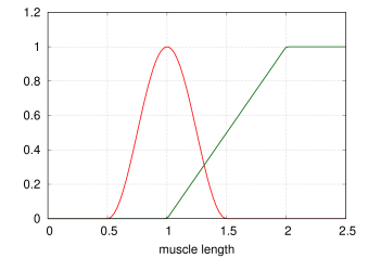 |
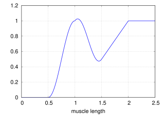 |
Given a normalized fibre length described by
| (4.5) |
and a normalized muscle length
| (4.6) |
the force generated by this material is:
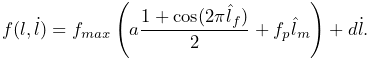 |
(4.7) |
The parameters are specified as properties of PeckAxialMuscle:
| Property | Description | Default | |
|---|---|---|---|
| maxForce | maximum contractile force | 1 | |
| passiveFraction | proportion of |
0 | |
| tendonRatio | tendon to fibre length ratio | 0 | |
| maxLength | length at which maximum passive force is generated | 1 | |
| optLength | length at which maximum active force is generated | 0 | |
| damping | damping parameter | 0 |
Figure 4.5 illustrates the force length relationship for a PeckAxialMuscle.
PeckAxialMuscles can be created with the following factory methods:
where fmax, lopt, lmax, tratio, pfrac
and damping specify ![]() ,
, ![]() ,
, ![]() ,
, ![]() ,
,
![]() and
and ![]() , and other properties are set to their defaults.
, and other properties are set to their defaults.
Creating a PeckAxialMuscle with the no-args constructor, or another constructor not listed above, will cause its forceScaling property (Section 4.5.1) to be set to 1000 instead of 1, thus requiring that fmax and damping be correspondingly reduced.
4.5.1.5 BlemkerAxialMuscle
The BlemkerAxialMuscle material generates a force as described in [5]. It is the axial muscle equivalent to the constitutive equation along the muscle fiber direction specified in the BlemkerMuscle FEM material.
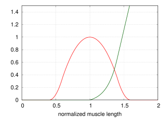 |
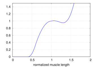 |
The force produced is a combination of active and passive terms, plus a damping term, given by
| (4.8) |
where ![]() is the maximum force,
is the maximum force, ![]() is the
normalized muscle length, and
is the
normalized muscle length, and
![]() and
and ![]() are the active and passive
force length curves, given by
are the active and passive
force length curves, given by
![f_{L}(\hat{l})=\begin{cases}9\,(\hat{l}-0.4),&\hat{l}\in[0.4,0.6]\\
1-4(1-\hat{l}),&\hat{l}\in[0.6,1.4]\\
9\,(\hat{l}-1.6),&\hat{l}\in[1.4,1.6]\\
0,&\mathrm{otherwise},\\
\end{cases}](mi/mi1889.png) |
(4.9) |
and
![f_{P}(\hat{l})=\begin{cases}0,&\hat{l}<1\\
P_{1}(e^{P_{2}(\hat{l}-1)}-1),&\hat{l}\in[l_{opt},l_{max}/l_{opt}]\\
P_{3}\hat{l}+P_{4},&\hat{l}>l_{max}/l_{opt}.\\
\end{cases}](mi/mi1891.png) |
(4.10) |
For the passive force length curve, ![]() and
and ![]() are computed to
provide linear extrapolation for
are computed to
provide linear extrapolation for ![]() . The other
parameters are specified by properties of BlemkerAxialMuscle:
. The other
parameters are specified by properties of BlemkerAxialMuscle:
| Property | Description | Default | |
|---|---|---|---|
| maxForce | the maximum contractile force | ||
| expStressCoeff | exponential stress coefficient | 0.05 | |
| uncrimpingFactor | fibre uncrimping factor | 6.6 | |
| maxLength | length at which passive force becomes linear | 1.4 | |
| optLength | length at which maximum active force is generated | 1 | |
| damping | damping parameter | 0 |
Figure 4.6 illustrates the force length relationship for a BlemkerAxialMuscle.
BlemkerAxialMuscles can be created with the following constructors,
where lmax, lopt, fmax, ecoef, and uncrimp specify ![]() ,
, ![]() ,
, ![]() ,
, ![]() ,
, ![]() and
and
![]() , and properties are otherwise set to their defaults.
, and properties are otherwise set to their defaults.
4.5.2 Example: muscle attached to a rigid body
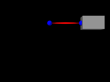
A simple model showing a single muscle connected to a rigid body is defined in
artisynth.demos.tutorial.SimpleMuscle
This model is identical to RigidBodySpring described in Section 3.2.2, except that the code to create the spring is replaced with code to create a muscle with a SimpleAxialMuscle material:
Also, so that the muscle renders differently, the rendering style for lines is set to SPINDLE using the convenience method
To run this example in ArtiSynth, select All demos > tutorial > SimpleMuscle from the Models menu. The model should load and initially appear as in Figure 4.7. Running the model (Section 1.5.3) will cause the box to fall and sway under gravity. To see the effect of the excitation property, select the muscle in the viewer and then choose Edit properties ... from the right-click context menu. This will open an editing panel that allows the muscle’s properties to be adjusted interactively. Adjusting the excitation property using the adjacent slider will cause the muscle force to vary.
4.5.3 Equilibrium muscles
ArtiSynth supplies several muscle materials that simulate a pennated
muscle in series with a tendon. Both the muscle and tendon generate
forces which are functions of their respective lengths ![]() and
and
![]() , and because these components are in series, their respective
forces must be equal when the system is in equilibrium. Given an
overall muscle-tendon length
, and because these components are in series, their respective
forces must be equal when the system is in equilibrium. Given an
overall muscle-tendon length ![]() , ArtiSynth solves
for
, ArtiSynth solves
for ![]() at each time step to ensure that this equilibrium condition
is met.
at each time step to ensure that this equilibrium condition
is met.

A general muscle-tendon system is illustrated by Figure
4.8, where ![]() and
and ![]() are the muscle and
tendon lengths. These two components generate forces given by
are the muscle and
tendon lengths. These two components generate forces given by
![]() and
and ![]() , where
, where ![]() , and the
fact that these components are in series implies that their forces
must be in equilibrium:
, and the
fact that these components are in series implies that their forces
must be in equilibrium:
| (4.11) |
The muscle force is in turn produced by a fibre force ![]() acting at a pennation angle
acting at a pennation angle ![]() with respect to the
principal muscle direction, such that
with respect to the
principal muscle direction, such that
where ![]() is the fibre length, which satisfies
is the fibre length, which satisfies
![]() , and
, and ![]() .
.
The fibre force is usually computed from the normalized fibre length
![]() and normalized fibre velocity
and normalized fibre velocity ![]() , defined by
, defined by
| (4.12) |
where ![]() is the optimal fibre length and
is the optimal fibre length and ![]() is the maximum
contraction velocity. It is composed of three components in parallel,
such that
is the maximum
contraction velocity. It is composed of three components in parallel,
such that
| (4.13) |
where ![]() is the maximum isometric force,
is the maximum isometric force,
![]() is the active force term induced by an
activation level
is the active force term induced by an
activation level ![]() and modulated by the active force length
curve
and modulated by the active force length
curve ![]() and the force velocity curve
and the force velocity curve ![]() ,
,
![]() is the passive force length curve, and
is the passive force length curve, and ![]() is an optional damping term induced by a fibre damping parameter
is an optional damping term induced by a fibre damping parameter
![]() .
.
The tendon force ![]() is computed from
is computed from
where ![]() is (again) the maximum isometric force,
is (again) the maximum isometric force, ![]() is the
tendon force length curve and
is the
tendon force length curve and ![]() is the normalized tendon
length, defined by dividing
is the normalized tendon
length, defined by dividing ![]() by the tendon slack length
by the tendon slack length
![]() :
:
As the muscle moves, it is assumed that the height ![]() from the fibre
origin to the main muscle line of action remains constant.
This height is defined by
from the fibre
origin to the main muscle line of action remains constant.
This height is defined by
where ![]() is the optimal pennation angle at the optimal
fibre length when
is the optimal pennation angle at the optimal
fibre length when ![]() .
.
4.5.4 Equilibrium muscle materials
The equilibrium muscle materials supplied by ArtiSynth include Thelen2003AxialMuscle and Millard2012AxialMuscle. These are all controlled by properties which specify the parameters presented in Section 4.5.3:
| Property | Description | Default | |
|---|---|---|---|
| maxIsoForce | maximum isometric force | 1000 | |
| optFibreLength | optimal fibre length | 0.1 | |
| tendonSlackLength | length beyond which tendon exerts force | 0.2 | |
| optPennationAngle | pennation angle at optimal fibre length (radians) | 0 | |
| maxContractionVelocity | maximum contraction velocity | 10 | |
| fibreDamping | damping parameter for normalized fibre velocity | 0 |
The materials differ from each other with respect to their active,
passive and tendon force length curves (![]() ,
, ![]() , and
, and
![]() ) and their force velocity curves (
) and their force velocity curves (![]() ).
).
For a given muscle instance, it is typically only necessary to specify
![]() ,
, ![]() ,
, ![]() and
and ![]() , where
, where ![]() ,
, ![]() and
and ![]() are given
in the model’s basic force and length units.
are given
in the model’s basic force and length units. ![]() is given in units
of
is given in units
of ![]() per second and has a default value of 10; changing this value
will stretch or contract the domain of the force velocity curve
per second and has a default value of 10; changing this value
will stretch or contract the domain of the force velocity curve
![]() . The damping parameter
. The damping parameter ![]() imparts a damping force
proportional to
imparts a damping force
proportional to ![]() and has a default value of 0 (i.e., no
damping). It is often not necessary to add fibre damping (since
damping can be readily applied to the model in other ways), but
and has a default value of 0 (i.e., no
damping). It is often not necessary to add fibre damping (since
damping can be readily applied to the model in other ways), but
![]() is supplied for formulations that do specify damping. If
non-zero,
is supplied for formulations that do specify damping. If
non-zero, ![]() is usually set to a value less than or equal to
is usually set to a value less than or equal to
![]() .
.
In addition to the above parameters, equilibrium muscle materials also export the following properties to adjust their behavior:
| Property | Description | Default |
|---|---|---|
| rigidTendon | forces the tendon to be rigid | false |
| ignoreForceVelocity | ignore the force velocity curve |
false |
If rigidTendon is true, the tendon will be assumed to be
rigid with a length given by the tendon slack length parameter ![]() .
This simplifies the muscle computations since
.
This simplifies the muscle computations since ![]() is then given by
is then given by
![]() and there is no need to compute an equilibrium position.
If ignoreForceVelocity is true, then force velocity
effects are ignored by replacing the force velocity curve
and there is no need to compute an equilibrium position.
If ignoreForceVelocity is true, then force velocity
effects are ignored by replacing the force velocity curve ![]() with
with ![]() .
.
The different equilibrium muscle materials are now summarized:
4.5.4.1 Millard2012AxialMuscle
Millard2012AxialMuscle implements the default version of the Millard2012EquilibriumMuscle model supplied by OpenSim [7] and described in [15].
The active, passive and tendon force length curves (![]() ,
,
![]() , and
, and ![]() ) and force velocity curve (
) and force velocity curve (![]() )
are implemented using cubic Hermite spline curves to conform closely
to the default curve values provided by OpenSim’s Millard2012EquilibriumMuscle. Plots of these curves are shown in
Figures 4.9 and 4.10. Both
the passive and tendon force curves are linearly extrapolated (and
hence exhibit constant stiffness) past
)
are implemented using cubic Hermite spline curves to conform closely
to the default curve values provided by OpenSim’s Millard2012EquilibriumMuscle. Plots of these curves are shown in
Figures 4.9 and 4.10. Both
the passive and tendon force curves are linearly extrapolated (and
hence exhibit constant stiffness) past ![]() and
and
![]() , respectively, with stiffness values of 2.857 and
29.06.
, respectively, with stiffness values of 2.857 and
29.06.
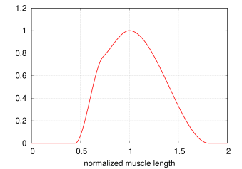 |
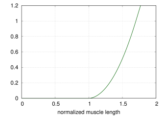 |
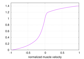 |
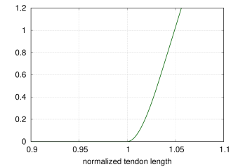 |
OpenSim requires that the Millard2012EquilibriumMuscle always exhibits a small bias activation, even when the activation should be zero, in order to avoid a singularity in the computation of the muscle length. ArtiSynth computes the muscle length in a manner that makes this unnecessary.
Millard2012AxialMuscles can be created using the constructors
where fmax, lopt, tslack, and optPenAng
specify ![]() ,
, ![]() ,
, ![]() , and
, and ![]() , and other properties are
set to their defaults.
, and other properties are
set to their defaults.
4.5.4.2 Thelen2003AxialMuscle
Thelen2003AxialMuscle implements the Thelen2003Muscle model supplied by OpenSim [7] and introduced in [27].
The active and passive force length curves are described by
| (4.14) |
and
| (4.15) |
where ![]() ,
, ![]() , and
, and ![]() are parameters, described
in [27], that control the curve shapes. These
are exposed as properties of Thelen2003AxialMuscle and are
described in Table 4.3.
are parameters, described
in [27], that control the curve shapes. These
are exposed as properties of Thelen2003AxialMuscle and are
described in Table 4.3.
The tendon force length curve is described by
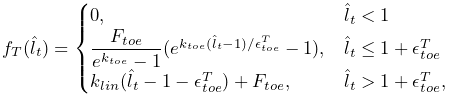 |
(4.16) |
where ![]() ,
, ![]() ,
, ![]() and
and ![]() are
parameters, described in [27], that control the
curve shape. The values of these are either fixed, or derived from the
maximum isometric tendon strain
are
parameters, described in [27], that control the
curve shape. The values of these are either fixed, or derived from the
maximum isometric tendon strain ![]() (controlled by the
fmaxTendonStrain property, Table 4.3),
according to
(controlled by the
fmaxTendonStrain property, Table 4.3),
according to
 |
(4.17) |
| Property | Description | Default | |
|---|---|---|---|
| kShapeActive | shape factor for active force length curve | 0.45 | |
| kShapePassive | shape factor for active force length curve | 5.0 | |
| fmaxMuscleStrain | passive muscle strain at maximum isometric muscle force | 0.6 | |
| fmaxTendonStrain | tendon strain at maximum isometric muscle force | 0.04 | |
| af | force velocity shape factor | 0.25 | |
| flen | maximum normalized lengthening force | 1.4 | |
| fvLinearExtrapThreshold |
|
0.95 |
The force velocity curve is determined from equation (6)
in [27]. In the notation used by that equation
and the accompanying equation (7), ![]() ,
, ![]() , and
, and ![]() . Inverting equation
(6) yields the force velocity curve:
. Inverting equation
(6) yields the force velocity curve:
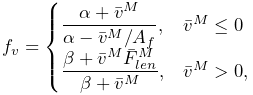 |
where
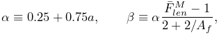 |
and ![]() is the activation level. Parameters include the maximum
normalized lengthening force
is the activation level. Parameters include the maximum
normalized lengthening force ![]() , and force velocity shape factor
, and force velocity shape factor
![]() , described in Table 4.3.
, described in Table 4.3.
Plots of the curves resulting from the above equations are shown, for default values, in Figures 4.11 and 4.12.
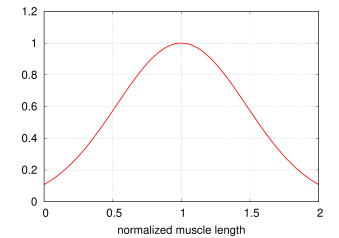 |
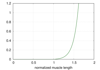 |
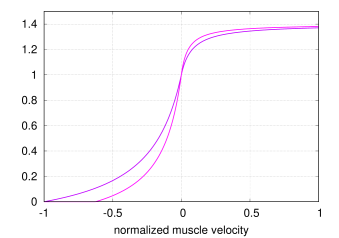 |
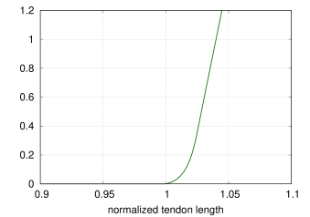 |
Thelen2003AxialMuscles can be created using the constructors
where fmax, lopt, tslack, and optPenAng
specify ![]() ,
, ![]() ,
, ![]() , and
, and ![]() , and other properties are
set to their defaults.
, and other properties are
set to their defaults.
4.5.5 Tendons and ligaments
Special point-to-point spring materials are also available to model tendons and ligaments. Because these are passive materials, they would normally be assigned to AxialSpring instead of Muscle components, although they will also work correctly in the latter. The materials include:
4.5.5.1 Millard2012AxialTendon
Millard2012AxialTendon implements the default tendon material of the Millard2012AxialMuscle (Section 4.5.4.1), with a force length relationship given by
| (4.18) |
where ![]() is the maximum isometric force,
is the maximum isometric force, ![]() is the tendon
force length curve (shown in Figure 4.10,
right), and
is the tendon
force length curve (shown in Figure 4.10,
right), and ![]() is the tendon slack length.
is the tendon slack length. ![]() and
and ![]() are specified
by the following properties of Millard2012AxialTendon:
are specified
by the following properties of Millard2012AxialTendon:
| Property | Description | Default | |
|---|---|---|---|
| maxIsoForce | maximum isometric force | 1000 | |
| tendonSlackLength | length beyond which tendon exerts force | 0.2 |
Millard2012AxialTendons can be created with the constructors
where fmax and tslack specify ![]() and
and ![]() , and
other properties are set to their defaults.
, and
other properties are set to their defaults.
4.5.5.2 Thelen2003AxialTendon
Thelen2003AxialTendon implements the default tendon material of the Thelen2003AxialMuscle (Section 4.5.4.2), with a force length relationship given by
| (4.19) |
where ![]() is the maximum isometric force,
is the maximum isometric force, ![]() is the tendon
force length curve described by equation (4.16),
and
is the tendon
force length curve described by equation (4.16),
and ![]() is the tendon slack length.
is the tendon slack length. ![]() ,
, ![]() , and the maximum
isometric tendon strain
, and the maximum
isometric tendon strain ![]() (used to determine the parameters
of (4.16), according to (4.17)),
are specified by the following properties of Thelen2003AxialTendon:
(used to determine the parameters
of (4.16), according to (4.17)),
are specified by the following properties of Thelen2003AxialTendon:
| Property | Description | Default | |
|---|---|---|---|
| maxIsoForce | maximum isometric force | 1000 | |
| tendonSlackLength | length beyond which tendon exerts force | 0.2 | |
| fmaxTendonStrain | tendon strain at maximum isometric muscle force | 0.04 |
Thelen2003AxialTendons can be created with the constructors
where fmax and tslack specify ![]() and
and ![]() , and
other properties are set to their defaults.
, and
other properties are set to their defaults.
4.5.5.3 Blankevoort1991AxialLigament
Blankevoort1991AxialLigament implements the Blankevoort1991Ligament model supplied by OpenSim [7] and described in [4, 24].
With the ligament strain and its derivative defined by
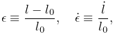 |
(4.20) |
the ligament force is given by
| (4.21) |
where
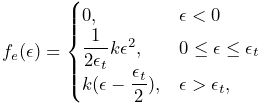 |
and
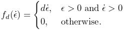 |
The parameters ![]() ,
, ![]() ,
, ![]() , and
, and ![]() are specified by the following
properties of Blankevoort1991Ligament:
are specified by the following
properties of Blankevoort1991Ligament:
| Property | Description | Default | |
|---|---|---|---|
| slackLength | ligament slack length | 0 | |
| transitionStrain | strain at transition from toe to linear | 0.06 | |
| linearStiffness | maximum stiffness of force-length curve | 100 | |
| damping | damping parameter | 0.003 |
Blankevoort1991Ligaments can be created with the constructors
where stiffness, slackLen and damping specify ![]() ,
,
![]() and
and ![]() , and other properties are set to their defaults.
, and other properties are set to their defaults.
4.5.6 Example: muscles with separate tendons
An alternate way to model the equilibrium muscles of Section
4.5.3 is to use two separate
point-to-point muscles, attached in series via a connecting particle
with a small mass (and possibly damping), thus implementing the muscle
and tendon components separately. This approach allows the muscle
equilibrium length to be determined automatically by the physical
response of the connecting particle, in a manner similar to that
employed by OpenSim’s Millard2012AccelerationMuscle (described
in [14]). For the muscle material, one
can use any of the tendonless materials of Section
4.5.1, or the materials of Section
4.5.3 with the properties rigidTendon and
tendonSlackLength set to true and ![]() , respectively, while
the tendon material can be one described in Section
4.5.5 or some other suitable passive material.
The implicit integrators used by ArtiSynth should permit relatively
stable simulation of the arrangement.
, respectively, while
the tendon material can be one described in Section
4.5.5 or some other suitable passive material.
The implicit integrators used by ArtiSynth should permit relatively
stable simulation of the arrangement.
While it is usually easier to employ the equilibrium muscle materials of Section 4.5.4, especially for models involving wrapping and/or via points (Chapter 9) where it may be difficult to handle the connecting particle correctly, in some situations the separate muscle/tendon method may offer a more versatile solution. It can also be used to validate the equilibrium muscles, as illustrated by the application model defined in
artisynth.demos.tutorial.EquilibriumMuscleDemo
which provides a direct comparison of the methods. It creates two simple instances of a Millard 2012 muscle, one above the other in the x-z plane, with the top instance implemented using the separate muscle/tendon method and the bottom instance implemented using an equilibrium muscle material (Figure 4.13). The application model uses control and monitoring components introduced in Chapter 5 to drive the simulation and record its results: a controller (Section 5.3) is used to uniformly extend the length of both muscles; output probes (Section 5.4) are used to record the resulting tension forces; and a control panel (Section 5.1) is created to allow the user to interactively adjust some of the muscle parameters.
The code for the EquilibriumMuscleDemo class attributes and build() method is shown below:
Lines 4-10 declare attributes for muscle parameters and the initial length of the combined muscle-tendon. Within the build() method, a MechModel is created with zero gravity (lines 14-16).
Next, the separate muscle/tendon muscle is assembled, consisting of
three particles (pl0, pc0, and pr0, lines 20-30), a
muscle mus0 connected between pl0 and pc0 (lines
33-39), and a tendon connected between pc0 and pr0
(lines 42-45). Particles pl0 and pr0 are both set to be
non-dynamic, since pl0 will be fixed and pr0 will be moved
parametrically, while the connecting particle pc0 has a small
mass and its position is updated by the simulation and so
automatically maintains force equilibrium between the muscle and
tendon. The material mat0 used for mus0 is an instance of
Millard2012AxialMuscle, with the tendon removed by setting the
tendonSlackLength and rigidTendon properties to ![]() and
true, respectively, while the material for tendon is an
instance of Millard2012AxialTendon.
and
true, respectively, while the material for tendon is an
instance of Millard2012AxialTendon.
The equilibrium muscle is then assembled, consisting of two particles (pl1 and pr1, lines 49-55) and a muscle mus1 connected between them (lines 57-61). pl1 and pr1 are both set to be non-dynamic, since pl1 will be fixed and pr1 will be moved parametrically, and the material mat1 for mus1 is an instance of Millard2012AxialMuscle in its default equilibrium mode. Excitations for both mus0 and mus1 are initialized to 1, and the zero-velocity equilibrium muscle length is computed using mat1.computeLmWithConstantVm() (lines 65-69). This is used to update the muscle position, for mus0 by setting the x coordinate of pc0 and for mus1 by setting the internal muscle length variable of mat1 (lines 71-72).
Render properties for different components are set at lines 76-80, and then a control panel is created to allow interactive adjustment of the muscle material properties optPennationAngle, fibreDamping, and ignoreForceVelocity, as well the muscle excitations (lines 83-88). As explained in Sections 5.1.1 and 5.1.3, addWidget() methods are used to create widgets that control each of these properties for both mus0 and mus1.
At line 92, a controller is added to the root model to move the
right side particles p0r and p1r during the simulation,
thus changing the muscles’ lengths and hence their tension
forces. Controllers are explained in Section
5.3, and the controller itself is defined
by lines 101-127 of the code listing below. At the start of each
simulation time step, the controller’s apply() method is called,
with t0 and t1 denoting the step’s start and end times.
It increases the x positions of p0r and p1r uniformly with
a speed of mySpeed until time myRunTime/2, and then
reverses direction until time myRunTime. Velocities are also
updated since these are needed to determine ![]() for the muscles’
computeF() methods.
for the muscles’
computeF() methods.
Each muscle’s tension force is recorded by an output probe connected to its forceNorm property. Probes are explained in Section 5.4; in this example, they are created using the convenience method addForceProbe(), defined by lines 130-140 (below) and called at lines 93-94 in the build() method, with probes for the muscle/tendon and equilibrium muscles named “muscle/tendon force” and “equilibrium force”, respectively.
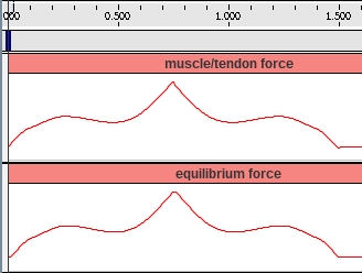 |
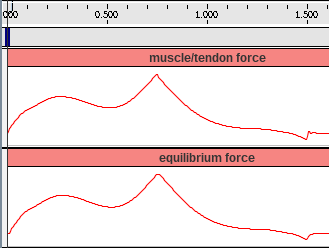 |
To run this example in ArtiSynth, select All demos > tutorial > EquilibriumMuscleDemo from the Models menu. The model should load and initially appear as in Figure 4.13. As explained above, running the model will cause the muscles to be extended and contracted by moving particles p0r and p1r right and back again. As this happens, the resulting tension forces can be examined by expanding the output probes in the timeline (see section “The Timeline” in the ArtiSynth User Interface Guide). The results are shown in Figure 4.14, with the left and right images showing results with the muscle material property ignoreForceVelocity set to true and false, respectively.
As should be expected, the results for the two muscle implementations are very similar. In both cases, the forces exhibit a local peak near time 0.25 when the muscle lengths are at the maximum of the active force length curve. As time increases, forces then decrease and then rise again as the passive force increases, peaking at time 0.75 when the muscle starts to contract. In the left image, the forces during contraction are symmetrical with those during extension, while in the right image the post-peak forces are more attenuated, because in the latter case the force velocity relationship is enabled as this reduces forces when a muscle is contracting.
4.6 Distance Grids and Components
Distance grids, implemented by the class DistanceGrid, are currently used in ArtiSynth for both collision handling (Section 8.4.2) and spring and muscle wrapping around general surfaces (Section 9.3). A distance grid is a regular three dimensional grid that is used to interpolate a scalar distance field and its associated normals. For collision handling and wrapping purposes, this distance function is assumed to be signed and is used to estimate the penetration depth and associated normal direction of a point within some 3D object.
A distance grid consists of ![]() evenly spaced
vertices partitioning a volume into
evenly spaced
vertices partitioning a volume into ![]() cuboid
cells, with
cuboid
cells, with
The grid has overall widths ![]() ,
, ![]() ,
, ![]() along each axis, so
that the widths of each cell are
along each axis, so
that the widths of each cell are ![]() ,
, ![]() ,
, ![]() .
.
Scalar distances and normal vectors are stored at each vertex, and
interpolated at points within each cell using trilinear interpolation.
Distance values (although not normals) can also be interpolated quadratically over a composite quadratic cell composed of ![]() regular cells. This provides a smoother result than
trilinear interpolation and is currently used for muscle wrapping. To
ensure that all points within the grid can be assigned a unique
quadratic cell, the grid resolution is restricted so that
regular cells. This provides a smoother result than
trilinear interpolation and is currently used for muscle wrapping. To
ensure that all points within the grid can be assigned a unique
quadratic cell, the grid resolution is restricted so that ![]() ,
,
![]() ,
, ![]() are always even. Distance grids are typically generated
automatically from mesh data. More details on the actual
functionality of distance grids is contained in
the DistanceGrid API documentation.
are always even. Distance grids are typically generated
automatically from mesh data. More details on the actual
functionality of distance grids is contained in
the DistanceGrid API documentation.
When used within ArtiSynth, distance grids are generally contained within an encapsulating DistanceGridComp component, which maintains a mesh (or list of meshes) used to generate the grid, and exports properties for controlling its resolution, mesh fit, and visualization. For any object that implements CollidableBody (which includes RigidBody), its distance grid component can be obtained using the method
A distance grid maintains its own local coordinate system, which is related to world coordinates by a local-to-world transform that can be queried and set via the component methods setLocalToWorld() and getLocalToWorld(). For grids associated with a rigid body, the local coordinate system is synchronized with the rigid body’s coordinate system (which is queried and set via setPose() and getPose()). The grid’s axes are nominally aligned with the local coordinate system, although they can be subject to an additional orientation offset (e.g., see the description of the property fitWithOBB below).
By default, a DistanceGridComp generates its grid automatically
from its mesh data, within an axis-aligned bounding volume with the
resolutions ![]() ,
, ![]() ,
, ![]() chosen automatically. However, in
some cases it may be necessary to control the resolution explicitly.
DistanceGridComp exports the following properties to control
both the grid’s resolution and how it is fit around the mesh data:
chosen automatically. However, in
some cases it may be necessary to control the resolution explicitly.
DistanceGridComp exports the following properties to control
both the grid’s resolution and how it is fit around the mesh data:
- resolution
-
A vector of 3 integers that specifies the resolutions
 ,
,  ,
,  . If any value in this vector is set
 , then all values are set to zero and
the maxResolution property is used to determine the grid
divisions instead.
, then all values are set to zero and
the maxResolution property is used to determine the grid
divisions instead. - maxResolution
-
Sets the default maximum cell resolution that should be used when constructing the grid. This is the number of cells that should be used along the longest bounding volume axis, with the cell counts along the other axes adjusted to maintain a uniform cell size. If all three values of resolution are
 , those
will be used to specify the cell resolutions instead.
, those
will be used to specify the cell resolutions instead. - fitWithOBB
-
If true, offsets the orientation of the grid’s x, y, and z axes (with respect to local coordinates) to align with an oriented bounding box fit to the mesh. Otherwise, the grid axes are aligned with those of the local coordinate frame.
- marginFraction
-
Specifies the fractional amount by which the mesh should be extended with respect to a bounding box fit around the mesh(es). The default value is 0.1.
As with all properties, these can be set either interactively (either using a custom control panel or by selecting the component and then choosing Edit properties ... from the right-click context menu), or through their set/get accessor methods. For example, resolution and maxResolution can be set and queried via the methods:
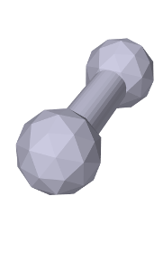 |
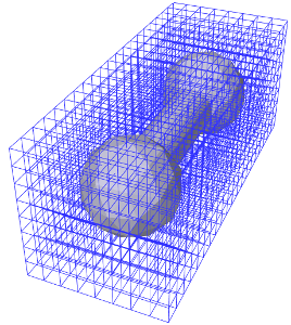 |
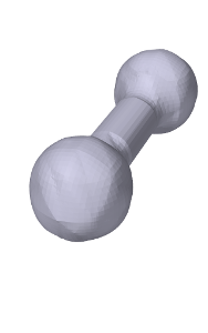 |
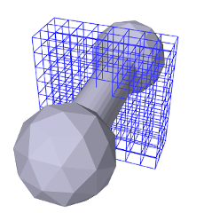 |
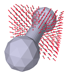 |
When used for either collisions or wrapping, the distance values interpolated by a distance grid are used to determine whether a point is inside or outside some 3D object, with the inside/outside boundary being the isosurface corresponding to a distance value of 0. This isosurface (which differs depending on whether trilinear or quadratic distance interpolation is used) therefore represents the effective collision boundary, and it may be somewhat different from the mesh surface used to generate it. It may be smoother, or may have discretization artifacts, depending on both the smoothness and complexity of the mesh and the grid’s resolution (Figure 4.15). It is therefore important to be able to visualize both the trilinear and quadratic isosurfaces. DistanceGridComp provides a number of properties to control this along with other aspects of grid visualization:
- renderProps
-
Render properties that control the colors, styles, and sizes (or widths) used to render faces, lines and points (Section 4.3). Point, line and edge properties are used for rendering grid vertices, normals, and cell edges, while face properties are used for rendering the isosurface. One can select which components are visible by zeroing appropriate render properties: zeroing pointRadius (or pointSize, if the pointStyle is POINT) disables drawing of the vertices; zeroing lineRadius (or lineWidth, if the lineStyle is LINE) disables drawing of the normals; and zeroing edgeWidth disables drawing of the cell edges. For an illustration, see Figure 4.16.
- renderGrid
-
If set to true, causes the grid’s vertices, normals and cell edges to be rendered, using the render properties as described above.
- renderRanges
-
Can be used to restrict which part of the distance grid is drawn. The value is a string which specifies the vertex ranges along the
, , and axes. In general, the grid will have  vertices along the , , and axes,
where
vertices along the , , and axes,
where  ,
,  , and
, and  are each one greater than the cell
resolutions , , and . The range string should contain
three range specifications, one for each axis, where each
specification is either * (all vertices), n:m (vertices in
the index range n to m, inclusive), or n (vertices
only at index n). A range specification of "* * *" (or
"*") means draw all vertices, which is the default
behavior. Other examples include:
are each one greater than the cell
resolutions , , and . The range string should contain
three range specifications, one for each axis, where each
specification is either * (all vertices), n:m (vertices in
the index range n to m, inclusive), or n (vertices
only at index n). A range specification of "* * *" (or
"*") means draw all vertices, which is the default
behavior. Other examples include:"* 7 *" all vertices along x and z, and those at index 7 along y "0 2 3" a single vertex at indices (0, 2, 3) "0:3 4:5 *" all vertices between 0 and 3 along x, and 4 and 5 along y
For an illustration, see Figure 4.16.
- renderSurface
-
If set to true, renders the grid’s isosurface, as determined by the surfaceType property. See Figure 4.15, right.
- surfaceType
-
Controls the interpolation used to form the isosurface rendered in response to the renderSurface property. QUADRATIC (the default) specifies a quadratic isosurface, while TRILINEAR specifies a trilinear isosurface.
- surfaceDistance
-
Controls the level set value used to determine the isosurface. To render the isosurface used for collision handling or muscle wrapping, this value should be 0.
When visualizing the isosurface for a distance grid, it is generally convenient to also turn off visualization for the meshes used to generate the grid. For RigidBody objects, this can be accomplished easily using the convenience property gridSurfaceRendering. If set true, it will cause the isosurface to be rendered instead of its mesh components. The isosurface type will be that indicated by the grid component’s surfaceType property, and the rendering will occur independently of the visibility settings for the meshes or the grid component.
4.7 Transforming geometry
Certain ArtiSynth components, including MechModel, implement the interface TransformableGeometry, which allows the geometric transformation of the component’s attributes (such as meshes, points, frame locations, etc.), along with its descendant components. The interface provides the method
where X is an AffineTransform3dBase that may be either a RigidTransform3d or a more general AffineTransform3d (Section 2.2).
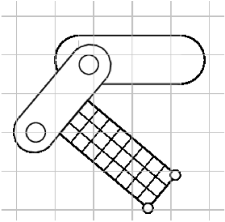 |
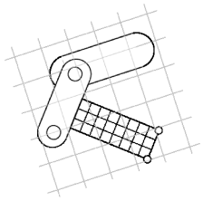 |
 |
transformGeometry(X) can be used to translate, rotate, shear or scale components. It can be applied to an entire model or individual components. Unlike scaleDistance(), it actually changes the physical geometry and so may change the simulation behavior. For example, applying transformGeometry() to a RigidBody will cause the shape of its mesh to change, which will change its mass if its inertiaMethod property is set to DENSITY. Figure 4.17 shows a simplified illustration of both rigid and affine transformations being applied to a model.
The example below shows how to apply a transformation to a model in code. In it, a MechModel is first scaled by the factors 1.5, 2, and 3 along the x, y, and z axes, and then flipped upside down using a RigidTransform3d that rotates it by 180 degrees about the x axis:
The transform specified to transformGeometry is in world coordinates. If the component being transformed has its own local coordinate frame (such as a rigid body), and one wants to specify the transform in that local frame, then one needs to convert the transform from local to world coordinates. Let
be the local coordinate frame, and let
and
be the transform in world and body coordinates, respectively. Then
and so
As an example of converting a transform to world coordinates, suppose
we wish to scale a rigid body by ![]() ,
, ![]() , and
, and ![]() along its local
axes. The transformation could then be done as follows:
along its local
axes. The transformation could then be done as follows:
4.7.1 Nonlinear transformations
The TransformableGeometry interface also supports general, nonlinear geometric transforms. This can be done using a GeometryTransformer, which is an abstract class for performing general transformations. To apply such a transformation to a component, one can create and initialize an appropriate subclass of GeometryTransformer to perform the desired transformation, and then apply it using the static transform method of the utility class TransformGeometryContext:
At present, the following subclasses of GeometryTransformer are available:
- RigidTransformer
-
Implements rigid 3D transformations.
- AffineTransformer
-
Implements affine 3D transformations.
- FemGeometryTransformer
-
Implements a general transformation, using the deformation field induced by a finite element model.
TransformGeometryContext also supplies the following convenience methods to apply transformations to components or collections of components:
The last three of these methods create an instance of either RigidTransformer or AffineTransformer for the supplied AffineTransform3dBase. In fact, most TransformableGeometry components implement their transformGeometry(X) method as follows:
The FemGeometryTransformer class is derived from the class DeformationTransformer, which uses the single method getDeformation() to obtain deformation field information at a specified reference position:
If the deformation field is described by ![]() , then
for a given reference position
, then
for a given reference position ![]() (in undeformed coordinates),
this method should return the deformed position
(in undeformed coordinates),
this method should return the deformed position ![]() and the deformation gradient
and the deformation gradient
| (4.22) |
evaluated at ![]() .
.
FemGeometryTransformer obtains
![]() and
and ![]() from a
FemModel3d (see Section
6) whose elemental rest positions enclose the
components to be transformed, using the fact that a finite element
model creates an implied piecewise-smooth deformation field as it
deviates from its rest position. For each reference point
from a
FemModel3d (see Section
6) whose elemental rest positions enclose the
components to be transformed, using the fact that a finite element
model creates an implied piecewise-smooth deformation field as it
deviates from its rest position. For each reference point ![]() needed
by the transformation process, FemGeometryTransformer finds the
FEM element whose rest volume encloses
needed
by the transformation process, FemGeometryTransformer finds the
FEM element whose rest volume encloses ![]() , and then uses the
corresponding shape function coordinates to compute
, and then uses the
corresponding shape function coordinates to compute ![]() and
and ![]() from the element’s deformation. If the FEM model does not
enclose
from the element’s deformation. If the FEM model does not
enclose ![]() , the nearest element is used to determine the shape
function coordinates (however, this calculation becomes less accurate and
meaningful the farther
, the nearest element is used to determine the shape
function coordinates (however, this calculation becomes less accurate and
meaningful the farther ![]() is from the FEM model). Transformations based
on FEM models are further illustrated in Section
4.7.2, and by Figure
4.19. Full details on ArtiSynth finite
element models are given in Section 6.
is from the FEM model). Transformations based
on FEM models are further illustrated in Section
4.7.2, and by Figure
4.19. Full details on ArtiSynth finite
element models are given in Section 6.
Besides FEM models, there are numerous other ways to create deformation fields, such as radial basis functions, thin plate splines, etc. Some of these may be more appropriate for a particular application and can provide deformations that are globally smooth (as opposed to piecewise smooth). It should be relatively easy for an application to create its own subclass of DeformationTransformer to implement the deformation of choice by overriding the single getDeformation() method.
4.7.2 Example: the FemModelDeformer class
An FEM-based geometric transformation of a MechModel is facilitated by the class FemModelDeformer, which one can add to an existing RootModel to transform the geometry of a MechModel already located within that RootModel. FemModelDeformer subclasses FemModel3d to include a FemGeometryTransformer, and provides some utility methods to support the transformation process.
A FemModelDeformer can be added to a RootModel by adding the following code fragment to the end of the build() method:
When the deformer is created, its constructor searches the specified RootModel to locate the first top-level MechModel. It then creates a hexahedral FEM grid around this model, with maxn specifying the number of cells along the maximum dimension. Material and mass properties of the model are computed automatically from the underlying MechModel dimensions (but can be altered if necessary after construction). When added to the RootModel, the deformer becomes another top-level model that can be deformed independently of the MechModel to create the required deformation field, as described below. It also supplies application-defined menu items that appear under the Application menu in the ArtiSynth menu bar (see Section 5.6). The deformer’s createControlPanel() can also be used to create a ControlPanel (Section 5.1) that controls the visibility of the FEM model and the dynamic behavior of both it and the MechModel.
An example is defined in
artisynth.demos.tutorial.DeformedJointedCollide
where the JointedCollide example of Section 8.1.3 is extended to include a FemModelDeformer using the code described above.
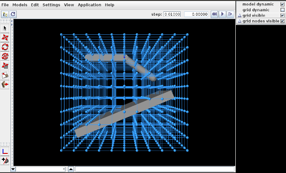
To load this example in ArtiSynth, select All demos > tutorial > DeformedJointedCollide from the Models menu. The model should load and initially appear as in Figure 4.18, where the control panel appears on the right.
The underlying MechModel (or "model") can now be transformed by first deforming the FEM model (or "grid") and then using the resulting deformation field to effect the transformation:
-
1.
Make the model non-dynamic and the grid dynamic by unchecking model dynamic and checking grid dynamic in the control panel. This means that when simulation is run, the model will be inert while the grid will respond physically.
-
2.
Deform the grid using simulation. One easy way to do this is to fix certain nodes, generally on or near the grid boundary, and then move some of these using the translation or transrotator tool while simulation is running. To fix a set of nodes, select them in the viewer, choose Edit properties ... from the right-click context menu, and then uncheck their dynamic property. To easily select a large number of nodes without also selecting model components or grid elements, one can specify FemNode in the selection filter widget. (See the sections “Transformer Tools” and “Selection filtering” in the ArtiSynth User Interface Guide.)
-
3.
After the grid has been deformed, choose deform from the Application menu in the ArtiSynth toolbar to transform the model. Afterwards, the transformation can be undone by choosing undo, and the grid can be reset by choosing reset grid.
-
4.
To run the deformed model after the transformation, it should again be made dynamic by checking model dynamic in the control panel. The grid itself can be made non-dynamic, and it and/or its nodes can be made invisible by unchecking grid visible and/or grid nodes visible in the control panel.
The result of a possible deformation is shown in Figure 4.19.
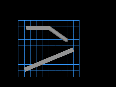 |
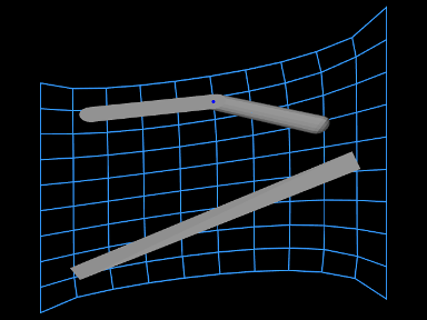 |
Note: FemModelDeformer is not intended to provide a general purpose solution to nonlinear geometric transformations. Rather, it is mainly intended to illustrate the capabilities of GeometryTransformer and the TransformableGeometry interface.
4.7.3 Implementation and behavior
As indicated above, the management of transforming the geometry for one or more components is handled by the TransformGeometryContext class. The transform operations themselves are carried out by this class’s apply() method, which (a) assembles all the components that need to be transformed, (b) performs the actual transform operations, (c) invokes any required updating actions on other components, and finally (d) notifies parent components of the change using a GeometryChangeEvent.
To support this, ArtiSynth components which implement TransformableGeometry must also supply the methods
The first method, addTransformableDependencies(context,flags), is called in step (a) to add to the context any additional components which should be transformed along with this component. This includes any descendants which should be transformed, since the transformation of these should not generally be done withintransformGeometry(gtr,context,flags).
The second method, transformGeometry(gtr,context,flags), is called in step (b) to perform the actual transformation on this component. It should use the supplied geometry transformer gtr to transform its attributes, as well as context to query what other components are also being transformed and to request any needed updating actions to be called in step (c). The flags argument specifies conditions associated with the transformation, which at the moment may currently include:
- TG_SIMULATING
-
The system is currently simulating, and therefore it may not be desirable to transform all attributes;
- TG_ARTICULATED
-
Rigid body articulation constraints should be enforced as the transform proceeds.
Full details for all this are given in the documentation for TransformGeometryContext.
The transforming behavior of a component is up to its implementing method, but the following rules are generally observed:
-
1.
Transformable descendants are also transformed, by using addTransformableDependencies() to add them to the context as described above;
-
2.
When the nodes of an FEM model (Section 6) are transformed, the rest positions are also transformed if the system is not simulating (i.e., if the TG_SIMULATING flag is not set). This also causes the mass of the adjacent nodes to be recomputed from the densities of the adjacent elements;
-
3.
When dynamic components are transformed, any attachments and constraints associated with them are updated appropriately, but only if the system is not simulating. Non-transforming dynamic components that are attached to transforming components are generally updated so as to follow the transforming components to which they are attached.
4.7.4 Use in model registration
Transforming model geometry can obviously be used as part of the process of creating subject-specific biomechanical and anatomical models. However, registration will generally require more than geometric transformation, since other properties, such as material stiffnesses, densities, and maximum forces will generally need to be adjusted as well. As a specific example, when applying a geometric transform to a model containing AxialSprings, the restLength properties of the springs will be unchanged, whereas the initial lengths may be, resulting in different applied forces and physical behavior.
4.8 General component arrangements
As discussed in Section 1.1.2 and elsewhere, a MechModel provides a number of predefined child components for storing particles, rigid bodies, springs, constraints, and other components. However, applications are not required to store their components in these containers, and may instead create any sort of component arrangement desired.
For example, suppose that one wishes to create a biomechanical model of both the right and left human arms, consisting of bones, point-to-point muscles, and joints. The standard containers supplied by MechModel would require that all the components be placed within the following containers:
Instead of this, one may wish to set up a more appropriate component hierarchy, such as
To do this, the application build() method can create the necessary hierarchy and then populate it with whatever components are desired. Before simulation begins (or whenever the model structure is changed), the MechModel will recursively traverse the component hierarchy and update whatever internal structures are needed to run the simulation.
4.8.1 Container components
The generic class ComponentList can be used as a container for model components of a specific type. It can be created using a declaration of the form
where Type is the class type of the components and name is the name for the container. Once the container is created, it should be added to the MechModel (or another internal container) and populated with child components of the specified type. For example,
creates two containers named "parts" and "frames" for storing components of type Particle and Frame, respectively, and adds them to a MechModel referenced by mech.
In addition to ComponentList, applications may use several "specialty" container types which are subclasses of ComponentList:
- RenderableComponentList
-
A subclass of ComponentList, that has its own set of render properties which can be inherited by its children. This can be useful for compartmentalizing render behavior. Note that it is not necessary to store renderable components in a RenderableComponentList; components stored in a ComponentList will be rendered too.
- PointList
-
A RenderableComponentList that is optimized for rendering points, and also contains its own pointDamping property that can be inherited by its children.
- PointSpringList
-
A RenderableComponentList designed for storing point-based springs. It contains a material property that specifies a default axial material that can be used by its children.
- AxialSpringList
-
A PointSpringList that is optimized for rendering two-point axial springs.
If necessary, it is relatively easy to define one’s own customized list by subclassing one of the other list types. One of the main reasons for doing so, as suggested above, is to supply default properties to be inherited by the list’s descendants.
A component list which declares ModelComponent as its type can be used to store any type of component, including other component lists. This allows the creation of arbitrary component hierarchies. Generally eitherComponentList<ModelComponent> or RenderableComponentList<ModelComponent> are best suited to implement hierarchical groupings.
4.8.2 Example: a net formed from balls and springs
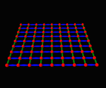
A simple example showing an arrangement of balls and springs formed into a net is defined in
artisynth.demos.tutorial.NetDemo
The build() method and some of the supporting definitions for this example are shown below.
The build() method begins by creating a MechModel in the usual way (lines 29-30). It then creates a net composed of a set of balls arranged as a uniform grid in the x-y plane, connected by a set of green colored springs running parallel to the y axis and a set of blue colored springs running parallel to the x axis. These are arranged into a component hierarchy of the form
using containers created at lines 37-42. The balls are then created and added to balls (lines 45-56), the springs are created and added to greenSprings and blueSprings (lines 59-71), and the containers are added to the MechModel at lines 74-77. The balls along the edges parallel to the y axis are fixed. Render properties are set at lines 80-83, with the colors for greenSprings and blueSprings being explicitly set to dark green and blue.
MechModel, along with other classes derived from ModelBase, enforces reference containment. That means that all components referenced by components within a MechModel must themselves be contained within the MechModel. This condition is checked whenever a component is added directly to a MechModel or one of its ancestors. This means that the components must be added to the MechModel in an order that ensures any referenced components are already present. For example, in the NetDemo example above, adding the particle list after the spring list would generate an error.
To run this example in ArtiSynth, select All demos > tutorial > NetDemo from the Models menu. The model should load and initially appear as in Figure 4.20. Running the model will cause the net to fall and sway under gravity. When the ArtiSynth navigation panel is opened and expanded, the component hierarchy will appear as in Figure 4.21. While the standard MechModel containers are still present, they are not displayed by default because they are empty.
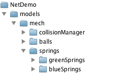
4.8.3 Adding containers to other models
In addition to MechModel, application-defined containers can be added to any model that inherits from ModelBase. This includes RootModel and FemModel. However, at the present time, components added to such containers won’t do anything, other than be rendered in the viewer if they are Renderable.
4.8.4 Reference lists for grouping components
It is sometimes useful to create groupings of model components in a manner that is both independent of their primary location within the model component hierarchy and also represented in the component hierarchy. However, it is not possible to do this using the ComponentList described in Section 4.8.1, since model components may only belong on one ComponentList (or more generally, one CompositeComponent) at a time.
Instead, one can use a ReferenceList, which contains references to a set of components of a particular type. Reference lists can be created with the constructors
| ReferenceList() |
Create an unnamed list. |
| ReferenceList(String name) |
Create a named list. |
Their definition is parameterized by the type of model component that they are intended to reference. For example, a reference list for components of type MeshComponent can be created and populated using the code fragment
To create a list that can accept any type of model component, simply parameterize it using ModelComponent:
Reference lists can be managed using the following methods, where C is the list’s component type:
| ReferenceComp addReference (C comp) |
Add a reference for comp. |
| void addReference (Collection<C> comps) |
Add references for each component in comps. |
| int numReferences() |
Get the number of references. |
| C getReference (int idx) |
Get the idx-th referenced component. |
| void getReferences (Collection<C> comps) |
Gets all referenced components. |
| boolean containsReference (C comp) |
Check if comp is referenced. |
| int indexOfReference (C comp) |
Get the index of the reference to comp. |
| boolean removeReference (C comp) |
Remove first reference to comp. |
| boolean removeReferences (Collection<C> comps) |
Remove all references to the components in comps. |
| void removeAllReferences () |
Remove all references. |
Internally, reference lists are implemented as component lists containing collections of ReferenceComp components that encapsulate each component reference. (The addReference() method returns the ReferenceComp that it creates for the added reference).
Unlike with component lists, a reference list may contain multiple references to the same component.
An application’s code base is of coarse free to create arbitrary collections of components using Java arrays or the various Collection classes defined in java.util. As indicated above, the purpose of a reference list is to incorporate such a collection into the component hierarchy, where it can be accessed from the navigation panel and will persist if the model is saved and reloaded.
4.8.5 Example: reference lists in NetDemo
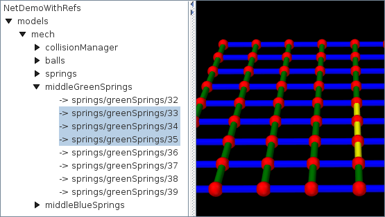
An extension to the NetDemo example of Section 4.8.2 that creates reference lists for subsets of the green and blue springs is defined in
artisynth.demos.tutorial.NetDemoWithRefs
The build() method is shown below:
Since the model is a subclass of NetDemo, the build() method begins
by creating the components of NetDemo with a call to super.build()
(line 2). Reference lists are then created to hold the green and blue springs
located in the middle of the net (lines 8-15). Each of these spring sets is
defined by indices ![]() with respect to the primary lists greenSprings and blueSprings. The lists are then added to the MechModel as direct subcomponents (lines 16-17).
with respect to the primary lists greenSprings and blueSprings. The lists are then added to the MechModel as direct subcomponents (lines 16-17).
Within the navigation panel, each component of a reference list is displayed as
-> path/to/reference
so that the referenced components are easy to locate. Selecting a reference in the panel selects the referenced component. Figure 4.22 shows NetDemoWithRefs with the navigation panel expanded to show the references for middleGreenSprings and three of the springs selected.
4.9 Custom Joints
If desired, it is also possible for applications to create their own custom joints. This involves creating two custom classes: a coupling class that does the constraint computations, and a joint class that wraps around it and allows it to connect connectable bodies. Details on how to create these classes are given in Sections 4.9.3 and 4.9.4, after some explanation of the constraint mechanism that underlies joint operation.
This section assumes that the reader is highly familiar with spatial kinematics and dynamics.
4.9.1 Joint constraints
To create a custom joint, it is necessary to understand how joints are
implemented. The basic function of a joint is to constrain the set of
poses allowed by the joint transform ![]() that relates frame C to
D. To do this, the joint imposes restrictions on the six-dimensional
spatial velocity
that relates frame C to
D. To do this, the joint imposes restrictions on the six-dimensional
spatial velocity ![]() that describes how frame C is moving
with respect to D. This restriction is done using a set of bilateral
constraints
that describes how frame C is moving
with respect to D. This restriction is done using a set of bilateral
constraints ![]() and (in some cases) unilateral constraints
and (in some cases) unilateral constraints ![]() ,
each of which is a
,
each of which is a ![]() matrix that acts to restrict a single
degree of freedom in
matrix that acts to restrict a single
degree of freedom in ![]() (see Section
A.5 for a review of
spatial velocities and forces). Bilateral constraints take the form of
an equality,
(see Section
A.5 for a review of
spatial velocities and forces). Bilateral constraints take the form of
an equality,
| (4.22) |
while unilateral constraints take the form of an inequality:
| (4.23) |
These constraints are defined with respect to frame C, and their total
number equals the number of DOFs that the joint removes. A
joint’s main computational task is to specify these
constraints. ArtiSynth then uses its own knowledge of how frames C and
D are connected to bodies A and B (or ground, if there is no body B)
to map the individual ![]() and
and ![]() onto the joint’s full
bilateral and unilateral constraint matrices
onto the joint’s full
bilateral and unilateral constraint matrices ![]() and
and ![]() (see
(3.4) and (3.5)) that restrict the
body velocities.
(see
(3.4) and (3.5)) that restrict the
body velocities.
As a simple example, consider a cylindrical joint, in which C is free
to rotate about and translate along the ![]() axis of D but other
motions are restricted. Letting
axis of D but other
motions are restricted. Letting ![]() and
and ![]() denote the
translational and rotational components of
denote the
translational and rotational components of ![]() , such that
, such that
we see that the constraints must enforce
| (4.24) |
This can be accomplished using four constraints defined as follows:
Constraining velocities is a necessary but insufficient condition for
constraint enforcement. Because of numerical errors, as well as the
fact that constraints are often nonlinear, the joint transform
![]() will tend to drift away from the joint restrictions as the
simulation proceeds, leading to the error
will tend to drift away from the joint restrictions as the
simulation proceeds, leading to the error ![]() described at the
end of Section 3.4.1. These errors are corrected
during a position correction at the end of every simulation time
step: the joint first projects
described at the
end of Section 3.4.1. These errors are corrected
during a position correction at the end of every simulation time
step: the joint first projects ![]() onto the nearest valid
constraint surface to form
onto the nearest valid
constraint surface to form ![]() , and
, and ![]() is then computed from
is then computed from
| (4.25) |
Because ![]() is (usually) small, we can approximate it as
a twist
is (usually) small, we can approximate it as
a twist ![]() representing a small displacement from frame
G (which lies on the constraint surface) to frame C. During the
position correction, ArtiSynth adjusts the pose of C relative to D in
order to try and bring
representing a small displacement from frame
G (which lies on the constraint surface) to frame C. During the
position correction, ArtiSynth adjusts the pose of C relative to D in
order to try and bring ![]() to zero. To do this, it uses
an estimate of the distance
to zero. To do this, it uses
an estimate of the distance ![]() along each constraint to the
constraint surface, which it computes from the dot product of
along each constraint to the
constraint surface, which it computes from the dot product of ![]() and
and ![]() :
:
| (4.26) |
ArtiSynth assembles these distances into a composite distance vector
![]() for all bilateral constraints, and then uses the system
solver to find a displacement
for all bilateral constraints, and then uses the system
solver to find a displacement ![]() of the system coordinates
that satisfies
of the system coordinates
that satisfies
Adding ![]() to the system coordinates
to the system coordinates ![]() then reduces the
constraint errors. While for nonlinear constraints several steps may be
required to bring the error to 0, the process usually converges
quickly.
then reduces the
constraint errors. While for nonlinear constraints several steps may be
required to bring the error to 0, the process usually converges
quickly.
Unlike bilateral constraints, unilateral constraints are one-sided,
and take effect, or are engaged, only when ![]() encounters
an inadmissible region. The constraint then acts to prevent further
penetration into the region, via the velocity restriction
(4.23), and also to push
encounters
an inadmissible region. The constraint then acts to prevent further
penetration into the region, via the velocity restriction
(4.23), and also to push ![]() out of the
inadmissible region, using a position correction analogous to that
used for bilateral constraints.
out of the
inadmissible region, using a position correction analogous to that
used for bilateral constraints.
Whether or not a unilateral constraint is engaged is determined by its
engaged value ![]() , which takes one of the three values:
, which takes one of the three values:
![]() , and is updated by the joint implementation as the
simulation proceeds. A value of 0 means that the constraint is not
engaged, and will not be included in the joint’s unilateral
constraint matrix
, and is updated by the joint implementation as the
simulation proceeds. A value of 0 means that the constraint is not
engaged, and will not be included in the joint’s unilateral
constraint matrix ![]() . Otherwise, if
. Otherwise, if ![]() is
is ![]() or
or ![]() , then the
constraint is engaged and will be included in
, then the
constraint is engaged and will be included in ![]() , using
, using ![]() if
if
![]() , or its negative
, or its negative ![]() if
if ![]() .
. ![]() therefore
defines a sign for the constraint. General details on how
unilateral constraints should be engaged or disengaged are discussed
in Section 4.9.2.
therefore
defines a sign for the constraint. General details on how
unilateral constraints should be engaged or disengaged are discussed
in Section 4.9.2.
A common use of unilateral constraints is to implement limits on joint
coordinate values; this also illustrates the utility of ![]() . For
example, the cylindrical joint mentioned above may have two
coordinates,
. For
example, the cylindrical joint mentioned above may have two
coordinates, ![]() and
and ![]() , describing the translation and rotation
along and about the D frame’s
, describing the translation and rotation
along and about the D frame’s ![]() axis. Now suppose we wish to bound
axis. Now suppose we wish to bound
![]() , such that
, such that
| (4.27) |
When these limits are violated, a unilateral constraint can be engaged
to limit motion along the ![]() axis.
A constraint
axis.
A constraint ![]() that will do this is
that will do this is
Whenever ![]() , using
, using ![]() in (4.23)
will ensure that
in (4.23)
will ensure that ![]() and hence
and hence ![]() will not fall further
below the lower bound. On the other hand, when
will not fall further
below the lower bound. On the other hand, when ![]() ,
we want to employ
,
we want to employ ![]() in (4.23) to ensure that
in (4.23) to ensure that
![]() . In other words, lower bounds can be enforced by
engaging
. In other words, lower bounds can be enforced by
engaging ![]() with
with ![]() , while upper bounds can be enforced
with
, while upper bounds can be enforced
with ![]() .
.
As with bilateral constraints, constraining velocities is not
sufficient; it is also necessary to correct position errors,
particularly as unilateral constraints are typically not engaged until
the inadmissible region is violated. The position correction procedure
is the same: for each engaged unilateral constraint, find a distance
![]() along its constraint direction that indicates the distance to
the inadmissible region boundary. ArtiSynth will then assemble these
along its constraint direction that indicates the distance to
the inadmissible region boundary. ArtiSynth will then assemble these
![]() into a composite distance vector
into a composite distance vector ![]() for all unilateral
constraints, and solve for a system coordinate displacement
for all unilateral
constraints, and solve for a system coordinate displacement ![]() that satisfies
that satisfies
| (4.28) |
Because of the inequality direction in
(4.28), distances ![]() representing
penetration into an inadmissible region must be negative. For
coordinate bounds such as (4.27), we need to use
representing
penetration into an inadmissible region must be negative. For
coordinate bounds such as (4.27), we need to use ![]() for the lower bound and
for the lower bound and ![]() for
the upper bound. Alternatively, if the unilateral constraint has been
included into the projection of C onto G and hence into the error term
for
the upper bound. Alternatively, if the unilateral constraint has been
included into the projection of C onto G and hence into the error term
![]() ,
, ![]() can be computed from
can be computed from
| (4.29) |
Note that unilateral constraints for coordinate limits are not
usually incorporated into the ![]() projection; more details on this are
given in Section 4.9.4.
projection; more details on this are
given in Section 4.9.4.
As simulation proceeds, the velocity limits imposed by
(4.22) and (4.23) are enforced by
bilateral and unilateral
constraint forces ![]() and
and ![]() whose
magnitudes are given by
whose
magnitudes are given by
| (4.30) |
where ![]() and
and ![]() are the Lagrange multipliers computed
by the mechanical system solver (and are components of
are the Lagrange multipliers computed
by the mechanical system solver (and are components of ![]() or
or
![]() in (1.10) and (1.13)).
in (1.10) and (1.13)).
![]() and
and ![]() are 6 DOF spatial force vectors, or wrenches
(Section A.5), which like
are 6 DOF spatial force vectors, or wrenches
(Section A.5), which like ![]() and
and
![]() are expressed in frame C. Because
are expressed in frame C. Because ![]() and
and ![]() are
proportional to spatial wrenches, they are often themselves referred
to as constraint wrenches, and within the ArtiSynth codebase are
described by a Wrench object.
are
proportional to spatial wrenches, they are often themselves referred
to as constraint wrenches, and within the ArtiSynth codebase are
described by a Wrench object.
4.9.2 Unilateral constraint engagement
As mentioned above, joints which implement unilateral constraints must
monitor ![]() and the joint coordinates as the simulation proceeds
and decide when to engage or disengage them.
and the joint coordinates as the simulation proceeds
and decide when to engage or disengage them.
Engagement is usually easy: a constraint is engaged whenever ![]() or a joint coordinate hits an inadmissible region. The constraint
or a joint coordinate hits an inadmissible region. The constraint
![]() is itself a spatial vector that is (locally) perpendicular to
the inadmissible region boundary, and
is itself a spatial vector that is (locally) perpendicular to
the inadmissible region boundary, and ![]() is chosen to be either
is chosen to be either
![]() or
or ![]() so that
so that ![]() is directed away from the
inadmissible region. In the remainder of this section, we shall assume
is directed away from the
inadmissible region. In the remainder of this section, we shall assume
![]() .
.
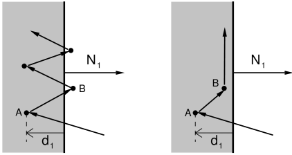
To disengage, we usually want to ensure that the joint configuration
is out of the inadmissible region. If we have a constraint ![]() ,
with a local distance
,
with a local distance ![]() defined such that
defined such that ![]() implies the
joint is inside the region, then we are out of the region when
implies the
joint is inside the region, then we are out of the region when
![]() . However, if we use only this as the disengagement
criterion, we may encounter a problem known as chattering,
illustrated in Figure 4.23 (left). An inadmissible
region is shown in gray, with a unilateral constraint
. However, if we use only this as the disengagement
criterion, we may encounter a problem known as chattering,
illustrated in Figure 4.23 (left). An inadmissible
region is shown in gray, with a unilateral constraint ![]() perpendicular to its boundary. As simulation proceeds, the joint lands
inside the region at an initial point A at the lower left, at a
(negative) distance
perpendicular to its boundary. As simulation proceeds, the joint lands
inside the region at an initial point A at the lower left, at a
(negative) distance ![]() from the boundary. Ideally the position
correction step will move the configuration by
from the boundary. Ideally the position
correction step will move the configuration by ![]() so that it lands
right on the region boundary. However, numerical errors and
nonlinearities may mean that in fact it lands outside the
region, at point B. Then on the next step it reenters the region, only
to again be pushed out, etc.
so that it lands
right on the region boundary. However, numerical errors and
nonlinearities may mean that in fact it lands outside the
region, at point B. Then on the next step it reenters the region, only
to again be pushed out, etc.
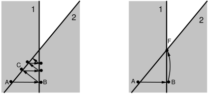
ArtiSynth implements two solutions to chattering. One is to implement
a deadband, so that instead of correcting the position by
![]() , we correct it by
, we correct it by ![]() , where
, where ![]() is a penetration tolerance. This means that the correction will
try to leave the joint inside the region by a small amount (Figure
4.23, right) so that chattering is suppressed. The
penetration tolerance used depends on the constraint type. Those that
are primarily linear use the value of the penetrationTol
property, while those that are primarily rotary use the value of the
rotaryLimitTol property; both of these are exported as
inheritable properties by both
MechModel and
BodyConnector, with default
values computed from the model’s overall dimensions.
is a penetration tolerance. This means that the correction will
try to leave the joint inside the region by a small amount (Figure
4.23, right) so that chattering is suppressed. The
penetration tolerance used depends on the constraint type. Those that
are primarily linear use the value of the penetrationTol
property, while those that are primarily rotary use the value of the
rotaryLimitTol property; both of these are exported as
inheritable properties by both
MechModel and
BodyConnector, with default
values computed from the model’s overall dimensions.
The second chattering solution is to disengage only when the joint is
actively moving away from the region, as determined by ![]() .
The disengagement criteria then become
.
The disengagement criteria then become
| (4.31) |
![]() is called the contact speed and can be computed from
is called the contact speed and can be computed from
| (4.32) |
Another problem, which we call constraint oscillation, can occur when we are near two or more overlapping inadmissible regions whose boundaries are not perpendicular. See Figure 4.24 (left), which shows two overlapping regions 1 and 2. The joint starts at point A, inside region 1 but just outside region 2. Since only constraint 1 is engaged, the position correction moves it toward the boundary of 1, overshooting and landing at point B outside of 1 but inside region 2. Constraint 2 now engages, moving the joint to C, where it is past the boundary of 2 but inside 1 again. While the example in the figure converges to the corner where the boundaries of 1 and 2 meet, convergence may be slow and may be prevented entirely by external forcing. While the mechanisms that prevent chattering may also prevent oscillation, we find that an additional measure is useful, which is to simply require that a constraint must be engaged for at least two simulation steps. The result is shown in Figure 4.24 (right), where after the joint arrives at B, constraint 1 remains engaged along with constraint 2, and the subsequent solution takes the joint directly to point F at the corner where 1 and 2 meet.
4.9.3 Implementing a custom joint
All of the work of computing joint constraints and coordinates, as described in the previous sections, is done within a “coupling” class which is a subclass of RigidBodyCoupling. An instance of this is then embedded within a “joint” class (which is a subclass of JointBase) that supports connections with other bodies, provides rendering, exports various properties, and allows the joint to be attached to a MechModel.
For purposes of this discussion, we will assume that these two custom classes are called CustomCoupling and CustomJoint, respectively. The implementation of CustomJoint can be as simple as this:
This creates an instance of CustomCoupling and sets it to the (inherited) myCoupling attribute inside the default constructor (which is where this normally should be done). Another constructor is provided which uses setBodies() to create a joint that is attached to two bodies with the D frame specified in world coordinates. In practice, a joint may also export some properties (such as joint coordinates), provide additional constructors, and implement rendering; one should examine the source code for some existing joints.
4.9.4 Implementing a custom coupling
Implementing a custom coupling constitutes most of the effort in
creating a custom joint, since the coupling is responsible for
maintaining the constraints ![]() and
and ![]() that enforce the joint
behavior.
that enforce the joint
behavior.
Before proceeding, we discuss the coordinate frame in which these
constraints are situated. It is often convenient to describe joint
constraints with respect to frame C, since rotations are frequently
centered there. However, the joint transform ![]() usually
contains errors (Section 3.4.1) due to a
combination of simulation error and possible joint compliance. To
determine these errors, we project C onto another frame G, defined to
be the nearest to C that is consistent with the bilateral (and possibly
some unilateral) constraints. (This is done by the projectToConstraints() method, described below). The result is a
joint transform
usually
contains errors (Section 3.4.1) due to a
combination of simulation error and possible joint compliance. To
determine these errors, we project C onto another frame G, defined to
be the nearest to C that is consistent with the bilateral (and possibly
some unilateral) constraints. (This is done by the projectToConstraints() method, described below). The result is a
joint transform ![]() that is “error free” with respect to
bilateral constraints and also consistent with the coordinates (if
supported). This makes it convenient to formulate constraints with
respect to frame G instead of C, and so this is the convention
ArtiSynth uses. In particular, the updateConstraints() method,
described below, uses
that is “error free” with respect to
bilateral constraints and also consistent with the coordinates (if
supported). This makes it convenient to formulate constraints with
respect to frame G instead of C, and so this is the convention
ArtiSynth uses. In particular, the updateConstraints() method,
described below, uses ![]() , together with the spatial velocity
, together with the spatial velocity
![]() describing the motion of G with respect to D.
describing the motion of G with respect to D.
An actual custom coupling implementation involves subclassing RigidBodyCoupling and then implementing five abstract methods, the outline of which looks like this:
The implementations of these methods are now described in detail.
initializeConstraints()
This method has the signature
and is called in the coupling’s superclass constructor (i.e., the constructor for RigidBodyCoupling). It is responsible for initializing the coupling’s constraints and (if supported) coordinates.
Constraints are added using one of the two superclass methods:
Each creates a new RigidBodyConstraint and adds it to the coupling’s constraint list. flags is an or-ed combination of the following flags defined in RigidBodyConstraint:
- BILATERAL
-
Constraint is bilateral (i.e., an equality). If BILATERAL is not specified, the constraint is considered unilateral.
- ROTARY
-
Constraint primarily restricts rotary motion. If it is unilateral, the joint’s rotaryLimitTol property is used for its penetration tolerance.
- LINEAR
-
Constraint primarily restricts translational motion. If it is unilateral, the joint’s penetrationTol property is used for its penetration tolerance.
- CONSTANT
-
Constraint is constant with respect to frame G. This flag is set automatically if the constraint is created using addConstraint(flags,wrench).
- LIMIT
-
Constraint is used to enforce limits for a coordinate. This flag is set automatically if the constraint is specified as the limit constraint for a coordinate.
The method addConstraint(flags,wrench) takes an additional Wrench argument specifying the (presumed constant) value of the constraint with respect to frame G, and sets the CONSTANT flag just described.
Coordinates are added similarly using using one of the two superclass methods:
Each creates a new CoordinateInfo object (which is an inner class
of RigidBodyCoupling), and adds it to the
coupling’s coordinate list. In the second method, min and max give
the initial range limits, and limCon, if non-null, specifies a
constraint (previously created using addConstraint) that is parallel to
the twist associated with the coordinate’s motion and which can be used for
enforcing the limits. Specifying a non-null limCon will cause the
constraint’s LIMIT flag to be set. The argument flags is reserved
for future use and should be set to 0. If not specified, the default coordinate
limits are ![]() .
.
Each coordinate is associated with a twist value which describes the instantaneous spatial velocity imparted by that coordinate in frame G. The twist value for each coordinate must be specified by the coupling, using the method
where cidx is the coordinate index and twistG is the current value of the twist expressed in coordinate frame G. If the twist has a constant value, setCoordinateTwist() may be called once in initializeConstraints(). Otherwise, it must be called in updateConstraints().
The implementation of initializeConstraints() for a coupling that implements a hinge type joint might look like this:
Six constraints are specified, with the sixth being a unilateral constraint that enforces the limits on the single coordinate describing the rotation angle. Each constraint and coordinate has an integer index giving the location in its list, in the order it was added. This index can be used to later retrieve the RigidBodyConstraint or CoordinateInfo object for the constraint or coordinate, using the methods getConstraint(idx) or getCoordinateInfo(idx).
Because initializeConstraints() is called in the superclass constructor, member attributes for the custom coupling will not yet be initialized when it is first called. Therefore, the method should not depend on the initial values of non-static member variables. initializeConstraints() can also be called later to rebuild the constraints if some defining setting is changed.
coordinatesToTCD()
This method has the signature
and is called when needed by the system. If coordinates are supported,
then the transform ![]() should be set from the coordinate values
supplied in coords, and returned in the argument TCD.
Otherwise, this method should do nothing.
should be set from the coordinate values
supplied in coords, and returned in the argument TCD.
Otherwise, this method should do nothing.
TCDToCoordinates()
This method has the signature
and is called when needed by the system. It is the inverse of coordinatesToTCD(): if coordinates are supported, then their values
should be set from the joint transform ![]() supplied by TCD
and returned in coords. Otherwise, this method should do
nothing.
supplied by TCD
and returned in coords. Otherwise, this method should do
nothing.
When calling this method, it is assumed that TCD is “legal” with respect to the joint’s constraints (as defined by projectToConstraints(), described next). If this is not the case, then projectToConstraints() should be called instead.
One issue that can arise is when a coordinate represents an angle
![]() that has a range greater than
that has a range greater than ![]() . In that case, a common
strategy is to compute a nominal value for
. In that case, a common
strategy is to compute a nominal value for ![]() , and then add or
subtract
, and then add or
subtract ![]() from it until the resulting value is as close as
possible to the current value for the angular coordinate. This
allows the angle to wrap through its entire range. To implement this,
one can use the method
from it until the resulting value is as close as
possible to the current value for the angular coordinate. This
allows the angle to wrap through its entire range. To implement this,
one can use the method
in the coordinate’s CoordinateInfo object, which finds the angle equivalent to phi that is nearest to the current coordinate value.
Coordinate values computed by this method should not be clipped to their ranges.
projectToConstraints()
This method has the signature
and is called when needed by the system. It is responsible for
projecting the joint transform ![]() (supplied by TCD) onto
the nearest transform
(supplied by TCD) onto
the nearest transform ![]() that is valid for the bilateral
constraints, and returning this in TGD. If coordinates are
supported and coords is non-null, then the coordinate
values corresponding to
that is valid for the bilateral
constraints, and returning this in TGD. If coordinates are
supported and coords is non-null, then the coordinate
values corresponding to ![]() should also be computed and returned
in coords. The easiest way to do this is to simply call TCDToCoordinates(TGD,coords), although in some cases it may be
computationally cheaper to compute both the coordinates and the
projection at the same time.
should also be computed and returned
in coords. The easiest way to do this is to simply call TCDToCoordinates(TGD,coords), although in some cases it may be
computationally cheaper to compute both the coordinates and the
projection at the same time.
Optionally, the coupling may also extend the projection to include
unilateral constraints that are not associated with coordinate
limits. In particular, this should be done for constraints for which
it is desired to have the constraint error included in ![]() and
the corresponding argument errC that is passed to updateConstraints().
and
the corresponding argument errC that is passed to updateConstraints().
updateConstraints()
This method has the signature
and is usually called once per simulation time step. It is responsible for:
-
•
Updating the values of all non-constant constraint wrenches, including the limit constraints for joint coordinates, along with their derivatives.
-
•
Updating the coordinate twists for couplings with joint coordinates, using the method setCoordinateTwist() described above. (For twists that are constant, setCoordinateTwist() can be called in initializeConstraints() instead.)
-
•
If updateEngaged is true, updating the engaged and distance attributes for all unilateral constraints not associated with a coordinate limit.
The method supplies several arguments:
-
•
TGD, containing the idealized joint transform
 from frame G to D produced by calling projectToConstraints().
-
•
TCD, containing the joint transform
from
frame C to D and supplied for legacy reasons. -
•
errC, representing the (hopefully small) error transform
 from frame C to G as a spatial twist vector.
 -
•
velGD, giving the spatial velocity
 of frame
G with respect to D, as seen in G; this is needed to compute wrench
derivatives.
of frame
G with respect to D, as seen in G; this is needed to compute wrench
derivatives. -
•
updateEngaged, which requests the updating of unilateral engaged and distance attributes as described above.
If the coupling supports coordinates, their values will be updated
before the method is called so as to correspond to ![]() . If
needed, a coordinate’s value may be obtained from the value
attribute of its CoordinateInfo object, which may in turn be
obtained using getCoordinateInfo(idx). Likewise, RigidBodyConstraint objects for each constraint may be obtained using
getConstraint(idx).
. If
needed, a coordinate’s value may be obtained from the value
attribute of its CoordinateInfo object, which may in turn be
obtained using getCoordinateInfo(idx). Likewise, RigidBodyConstraint objects for each constraint may be obtained using
getConstraint(idx).
Constraint wrenches correspond to ![]() and
and ![]() in Section
4.9.1. These, along with their derivatives
in Section
4.9.1. These, along with their derivatives
![]() and
and ![]() , are described by the wrenchG and dotWrenchG attributes of each constraint’s
RigidBodyConstraint object, and may
be managed by a variety of methods:
, are described by the wrenchG and dotWrenchG attributes of each constraint’s
RigidBodyConstraint object, and may
be managed by a variety of methods:
dotWrenchG is used in computing the constraint offset terms
and
that appear in (3.3) and (1.13). While these improve the computational accuracy of the simulation, their effect is often small, and so in practice one may be able to omit computing dotWrenchG and instead leave its value as 0.
Wrench information must also be computed for unilateral constraints
which implement coordinate limits. While it is not necessary to
compute the distance and engaged attributes for these
constraints (this is done automatically), it is necessary to
ensure that the wrench’s magnitude is compatible with the coordinate’s
speed. More precisely, if the coordinate is given by ![]() , then the
limit wrench
, then the
limit wrench ![]() must have a magnitude such that
must have a magnitude such that
| (4.33) |
As mentioned above, if updateEngaged is true, the engaged and distance attributes for unilateral constraints not
associated with coordinate limits must be updated. These correspond
to ![]() and
and ![]() in Section 4.9.1, and are
contained in the constraint’s
RigidBodyConstraint object and may
be queried using the methods
in Section 4.9.1, and are
contained in the constraint’s
RigidBodyConstraint object and may
be queried using the methods
It is up to updateConstraints() to compute the distance, with
a negative value denoting penetration into the inadmissible
region. If projectToConstraints() is
implemented so as to account for the constraint, then ![]() will
be projected out of the inadmissible region and the distance will be
implicitly present in
will
be projected out of the inadmissible region and the distance will be
implicitly present in ![]() and so can be recovered by taking
the dot product of the constraint wrench and velGD:
and so can be recovered by taking
the dot product of the constraint wrench and velGD:
Otherwise, if the constraint is not accounted for in projectToConstraints(), the distance must be obtained by other means.
To update engaged, one may use the general convenience method
which sets engaged according to the rules of Section 4.9.2, for an inadmissible region corresponding to dist < dmin or dist > dmax. The upper or lower bounds may be removed by setting dmin to -inf or dmax to inf, respectively.
4.9.5 Example: a simple custom joint
|
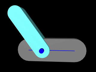 |
A simple model illustrating custom joint creation is provided by
artisynth.demos.tutorial.CustomJointDemo
This implements a joint class defined by CustomJoint (also in the package artisynth.demos.tutorial), which is actually just a simple implementation of SlottedHingeJoint (Section 3.5.4). Certain details are omitted, such as exporting coordinate values and ranges as properties, and other things are simplified, such as the rendering code. One may consult the source code for SlottedHingeJoint to obtain a more complete example.
This section will focus on the implementation of the joint coupling, which is created as an inner class of CustomJoint called CustomCoupling and which (like all couplings) extends RigidBodyCoupling. The joint itself creates an instance of the coupling in its default constructor, exactly as described in Section 4.9.3.
The coupling allows two DOFs (Figure 4.25, left):
translation along the ![]() axis of D (described by the coordinate
axis of D (described by the coordinate ![]() ),
and rotation about the
),
and rotation about the ![]() axis of D (described by the coordinate
axis of D (described by the coordinate
![]() ), with
), with ![]() related to the coordinates by
(3.19). It implements
initializeConstraints() as follows:
related to the coordinates by
(3.19). It implements
initializeConstraints() as follows:
Six constraints are added using addConstraint(): two linear bilaterals to
restrict translation along the ![]() and
and ![]() axes of D, two rotary bilaterals to
restrict rotation about the
axes of D, two rotary bilaterals to
restrict rotation about the ![]() and
and ![]() axes of D, and two unilaterals to
enforce limits on
axes of D, and two unilaterals to
enforce limits on ![]() and
and ![]() . Four of the constraints are constant in
frame G, and so are initialized with a wrench value. The other two are not
constant in G and so will need to be updated in updateConstraints(). The
coordinates for
. Four of the constraints are constant in
frame G, and so are initialized with a wrench value. The other two are not
constant in G and so will need to be updated in updateConstraints(). The
coordinates for ![]() and
and ![]() are added at the end, using addCoordinate(), with default joint limits and a reference to the constraint
that will enforce the limit. The twist for
are added at the end, using addCoordinate(), with default joint limits and a reference to the constraint
that will enforce the limit. The twist for ![]() is constant and so it is
initialized here as well.
is constant and so it is
initialized here as well.
The implementations for coordinatesToTCD() and TCDToCoordinates() simply use (3.19) to
compute ![]() from the coordinates, or vice versa:
from the coordinates, or vice versa:
X_IDX and THETA_IDX are constants defining the
coordinate indices for ![]() and
and ![]() . In TCDToCoordinates(),
note the use of the CoordinateInfo method nearestAngle(), as discussed in Section
4.9.4.
. In TCDToCoordinates(),
note the use of the CoordinateInfo method nearestAngle(), as discussed in Section
4.9.4.
Projecting ![]() onto the error-free
onto the error-free ![]() is done by projectToConstraints(), implemented as follows:
is done by projectToConstraints(), implemented as follows:
The translational projection is easy - the y and z components of the
translation vector p are simply zeroed out. To project the
rotation R, we use its rotateZDirection() method, which
applies the shortest rotation aligning its ![]() axis with
axis with ![]() . The residual rotation will be a rotation in the
. The residual rotation will be a rotation in the ![]() -
-![]() plane.
If coords is non-null and needs to be computed, we simply
call TCDToCoordinates().
plane.
If coords is non-null and needs to be computed, we simply
call TCDToCoordinates().
Lastly, the implementation for updateConstraints() is as follows:
Only constraints 0 and 4 need to have their wrenches updated, since
the rest are constant, and we obtain their constraint objects using
getConstraint(idx). Constraint 0 restricts motion along the ![]() axis in D, and while this is constant in D, it is not constant
in G, which is where the wrench must be situated. The
axis in D, and while this is constant in D, it is not constant
in G, which is where the wrench must be situated. The ![]() axis of D
as seen in G is the given by the second row of the rotation matrix of
axis of D
as seen in G is the given by the second row of the rotation matrix of
![]() , which from (3.19) we see is
, which from (3.19) we see is
![]() , where
, where ![]() and
and
![]() . We obtain
. We obtain ![]() and
and ![]() directly from TGD, since this has been projected to lie on the constraint surface;
alternatively, we could compute them from
directly from TGD, since this has been projected to lie on the constraint surface;
alternatively, we could compute them from ![]() . To obtain the
wrench derivative, we note that
. To obtain the
wrench derivative, we note that ![]() and
and
![]() , and that
, and that ![]() is simply the
is simply the ![]() component of the angular velocity of
component of the angular velocity of ![]() with respect to
with respect to ![]() , or velGD.w.z. The wrench and its derivative are set using the
constraint’s setWrenchG() and setDotWrenchG() methods.
, or velGD.w.z. The wrench and its derivative are set using the
constraint’s setWrenchG() and setDotWrenchG() methods.
The other non-constant constraint is the limit constraint for the ![]() coordinate, which is the
coordinate, which is the ![]() axis of D as seen in G. This is updated
similarly. Since all unilateral constraints are coordinate limits, there is no
need to update their distance or engaged attributes as this is done
automatically by the system.
axis of D as seen in G. This is updated
similarly. Since all unilateral constraints are coordinate limits, there is no
need to update their distance or engaged attributes as this is done
automatically by the system.
Finally, we use setCoordinateTwist() to update the twist for the ![]() coordinate, which is the spatial velocity imparted by a change in
coordinate, which is the spatial velocity imparted by a change in ![]() as seen
in frame G. Although this twist has the constant value
as seen
in frame G. Although this twist has the constant value ![]() in
frame D, it varies in frame G according to the transform from
in
frame D, it varies in frame G according to the transform from ![]() to
to ![]() . In
this particular example, it has the same values as the
. In
this particular example, it has the same values as the ![]() limit constraint.
limit constraint.
Chapter 5 Simulation Control
This section describes different devices which an application may use to control the simulation. These include control panels to allow for the interactive adjustment of properties, as well as agents which are applied every time step. Agents include controllers and input probes to supply and modify input parameters at the beginning of each time step, and monitors and output probes to observe and record simulation results at the end of each time step.
5.1 Control Panels
A control panel is an editing panel that allows for the interactive adjustment of component properties.
It is always possible to adjust component properties through the GUI by selecting one or more components and then choosing Edit properties ... in the right-click context menu. However, it may be tedious to repeatedly select the required components, and the resulting panels present the user with all properties common to the selection. A control panel allows an application to provide a customized editing panel for selected properties.
If an application wishes to adjust an attribute that is not exported as a property of some ArtiSynth component, it is often possible to create a custom property for the attribute in question. Custom properties are described in Section 5.2.
5.1.1 General principles
Control panels are implemented by the ControlPanel model component. They can be set up within a model’s build() method by creating an instance of ControlPanel, populating it with widgets for editing the desired properties, and then adding it to the root model using the latter’s addControlPanel() method. A typical code sequence looks like this:
There are various addWidget() methods available for adding widgets and components to a control panel. Two of the most commonly used are:
The first method creates a widget to control the property located by propPath with respect to the property’s host (which is usually a model component or a composite property). Property paths are discussed in Section 1.4.2, and can consist of a simple property name, a composite property name, or, for properties located in descendant components, a component path followed by a colon ‘:’ and then a simple or compound property name.
The second method creates a slider widget to control a property whose value is a single number, with an initial numeric range given by max and min.
The first method will also create a slider widget for a property whose value is a number, if the property has a default range and slider widgets are not disabled in the property’s declaration. However, the second method allows the slider range to be explicitly specified.
Both methods also return the widget component itself, which is an instance of LabeledComponentBase, and assign the widget a text label that is the same as the property’s name. In some situations, it is useful to assign a different text label (such as when creating two widgets to control the same property in two different components). For those cases, the methods
allow the widget’s text label to be explicitly specified.
Sometimes, it is desirable to create a widget that controls that same property across two or more host components (as illustrated in Section 5.1.3 below). For that, the methods
allow multiple hosts to be specified using the variable length argument list hosts.
Other flavors of addWidget() also exist, as described in the API documentation for ControlPanel. In particular, any type of Swing or awt component can be added using the method
Control panels can also be created interactively using the GUI; see the section “Control Panels” in the ArtiSynth User Interface Guide.
5.1.2 Example: Creating a simple control panel
An application model showing a control panel is defined in
artisynth.demos.tutorial.SimpleMuscleWithPanel
This model simply extends SimpleMuscle (Section 4.5.2) to provide a control panel for adjusting gravity, the mass and color of the box, and the muscle excitation. The class definition, excluding import statements, is shown below:
The build() method calls super.build() to create the model used by SimpleMuscle. It then proceeds to create a ControlPanel, populate it with widgets, and add it to the root model (lines 8-15). The panel is given the name "controls" in the constructor (line 8); this is its component name and is also used as the title for the panel’s window frame. A control panel does not need to be named, but if it is, then that name must be unique among the control panels.
Lines 9-11 create widgets for three properties located relative to the MechModel referenced by mech. The first is the MechModel’s gravity. The second is the mass of the box, which is a component located relative to mech by the path name (Section 1.1.5) "rigidBodies/box". The third is the box’s face color, which is the sub-property faceColor of the box’s renderProps property.
Line 12 adds a JSeparator to the panel, using the addWidget() method that accepts general components, and line 13 adds a widget to control the excitation property for muscle.
It should be noted that there are different ways to specify target properties in addWidget(). First, component paths may contain numbers instead of names, and so the box’s mass property could be specified using "rigidBodies/0:mass" instead of "rigidBodies/box:mass" since the box’s number is 0. Second, if a reference to a subcomponent is available, one can specify properties directly with respect to that, instead of indicating the subcomponent in the property path. For example, if the box was referenced by a variable body, then one could use the construction
panel.addWidget (body, "mass");in place of
panel.addWidget (mech, "rigidBodies/box:mass");
To run this example in ArtiSynth, select All demos > tutorial > SimpleMuscleWithPanel from the Models menu. The demo will appear with the control panel shown in Figure 5.1, allowing the displayed properties to be adjusted interactively by the user while the model is either stationary or running.
Double-clicking (using the left mouse button) on the label of a control panel widget will cause the component hosting that widget’s property to be selected. The path of the selected component will appear in the selection display beneath the viewer (see the section “Selection display” in the ArtiSynth User Interface Guide), and a context menu can be invoked for the component by right-clicking (or equivalent) within the viewer itself.
As described in Section 1.4.3, some properties are inheritable, meaning that their values can either be set explicitly within their host component, or inherited from the equivalent property in an ancestor component. Widgets for inheritable properties include an icon in the left margin indicating whether the value is explicitly set (square icon) or inherited from an ancestor (triangular icon) (Figure 5.1). These settings can be toggled by clicking on the icon. Changing an explicit setting to inherited will cause the property’s value to be changed to that of the nearest ancestor component, or to the property’s default value if no ancestor component contains an equivalent property.
5.1.3 Example: Controlling properties in multiple components
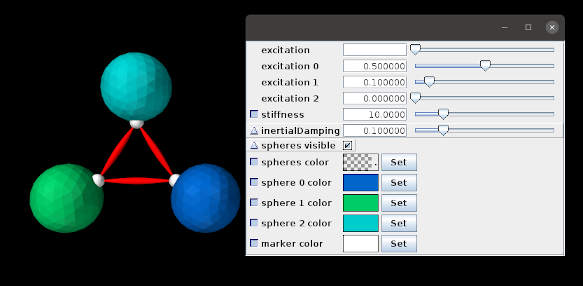
It is sometimes useful to create a property widget that adjusts the same property across several different components at the same time. This can be done using the addWidget() methods that accept multiple hosts. An application model demonstrating this is defined in
artisynth.demos.tutorial.ControlPanelDemo
and shown in Figure 5.2. The model creates a simple arrangement of three spheres, connected by point-to-point muscles and with collisions enabled (Chapter 8), whose dynamic behavior can be adjusted using the control panel. Selected rendering properties can also be changed using the panel. The class definition, excluding import statements, is shown below:
First, a MechModel is created with zero gravity and a default inertialDamping of 0.1 (lines 18-21). Next, three spheres are created, each with a different color and a frame marker attached to the top. These are positioned around the world coordinate origin, and oriented with their tops pointing toward the origin (lines 26-47), allowing them to be connected, via their markers, with three simple muscles (lines 49-52) created using the support method attachMuscle() (lines 8-14). Collisions (Chapter 8) are then enabled between all spheres (line 55).
At lines 62-64, we explicitly set the render properties for each marker; this is done because marker render properties are null by default and hence need to be explicitly set to enable widgets to be created for them, as discussed further below.
Finally, a control panel is created for various dynamic and rendering properties. These include the excitation and material stiffness for all muscles (lines 71 and 75); the inertialDamping, rendering visibility and faceColor for all spheres (lines 77, 79, and 81); and the rendering pointColor for all markers (line 85). The panel also allows muscle excitations and sphere face colors to be set individually (lines 72-74 and 82-84). Some of the addWidget() calls explicitly set the label text for their widgets. For example, those controlling individual muscle excitations are labeled as “excitation 0”, “excitation 1”, and “excitation 2” to denote their associated muscle.
Some widgets are created for subproperties of their components (e.g., material.stiffness and renderProps.faceColor). The following caveats apply in these cases:
-
1.
The parent property (e.g., renderProps for renderProps.faceColor) must be present in the component. While this will generally be true, in some instances the parent property may have a default value of null, and must be explicitly set to a non-null value before the widget is created (otherwise the subproperty will not be found and the widget creation will fail). This most commonly occurs for the renderProps property of smaller components, like particles and markers; in the example, render properties are explicitly assigned to the markers at lines 62-64.
-
2.
If the parent property is changed for a particular host, then the widget will no longer be able to access the subproperty. For instance, in the example, if the material property for a muscle is changed (via either code or the GUI), then the widget controlling material.stiffness will no longer be able to access the stiffness subproperty for that muscle.
To run this example in ArtiSynth, select All demos > tutorial > ControlPanelDemo from the Models menu. When the model is run, the spheres will start to be drawn together by the muscles’ intrinsic stiffness. Setting non-zero excitation values in the control panel will increase the attraction, while setting stiffness values will likewise affect the dynamics. The panel can also be used to make all the spheres invisible, or to change their colors, either separately or collectively.
When a single widget is used to control a property across multiple host components, the property’s value may not be the same for those components. When this occurs, the widget’s value field displays either blank space (for numeric, string and enum values), a “?” (for boolean values), or a checked pattern (for color values). This is illustrated in Figure 5.2 for the “excitation” and “spheres color” widgets, since their individual values differ.
5.1.4 Coordinate panels
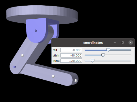
A special subclass of ControlPanel is a CoordinatePanel, which supports the addition of widgets for controlling joint coordinate values. A CoordinatePanel is associated with the MechModel containing the coordinates’ joints. When a coordinate value changes, the MechModel is used to update other model components that may be affected, such as the wrap paths for MultiPointSprings and the locations of attached components.
At present, CoordinatePanels do not take into account couplings between coordinate values that may be induced by kinematic loops within the model. This will be remedied in the future.
A CoordinatePanel may be created with the constructor
| CoordinatePanel (String name, MechModel mech) |
which assigns it a name and MechModel. Coordinate widgets may then be added using a variety of methods:
The first three methods create a coordinate widget for a given joint, with the coordinate itself specified by either its name (cname) or index (cidx). For the third method, the widget’s label can be set explicitly; if label is null, or unspecified as in the other methods, then a label is generated from the coordinate’s name. The next four methods specify the coordinate using a JointCoordinateHandle, which encapsulates both a coordinate’s joint and index information and can be constructed easily as follows:
Some of these methods also allow the widget’s value range to be explicitly set via the arguments min and max. The final method, addCoordinateWidgets() adds widgets for every coordinate within the specified joint.
These methods return CoordinateWidget, which is a subclass of DoubleFieldSlider. Other types of widgets may be added to a CoordinatePanel using the addWidget() methods inherited from ControlPanel.
CoordinatePanel widgets represent their values for revolute coordinates in degrees.
When added to the example MultiJointedArm (Section 3.5.16), the following code fragment creates the coordinate panel shown in Figure 5.3:
Double-clicking (using the left mouse button) on the label of a coordinate widget will cause the joint associated with that coordinate to be selected. The joint’s component path will appear in the selection display beneath the viewer, and a context menu can be invoked by right-clicking (or equivalent) within the viewer itself. Choosing “Edit properties ...” from the context menu will create a property dialog for the joint, allowing other coordinate properties, such as its range and whether or not it is locked, to be set.
5.1.4.1 Panel settings
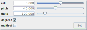
Once a coordinate panel is created, an application can use the method addSettingsPanel() to add a subpanel that controls the panel’s behavior:
The panel, shown in Figure 5.4, controls the following behavior settings:
-
•
Degrees: Sets whether values for rotary coordinates are expressed in degrees. The default setting is true.
-
•
Multiset: If true, changing the widget values does not change the underlying coordinates until the panel’s Set button is clicked, at which point all change requests are applied at once. This allows multiple coordinate values to be set simultaneously.
The degrees setting can also be controlled in code using the methods
| boolean getUseDegrees() |
Queries use of degrees for rotary coordinates. |
| void setUseDegrees (boolean enable) |
Sets use of degrees for rotary coordinates. |
5.1.4.2 Coordinate setting methods
For convenience, CoordinatePanel offers access to its underlying CoordinateSetter, together with wrapper methods to set or get coordinate values based on the widget label:
| CoordinateSetter getCoordinateSetter() |
Get the underlying coordinate setter. |
| double getCoordinate (String label) |
Get value by widget label (radians for rotary coords). |
| SetStatus setCoordinate (String label, double val) |
Set value by widget label (radians for rotary coords). |
| double getCoordinateDeg (String label) |
Get value by widget label (degrees for rotary coords). |
| SetStatus setCoordinateDeg (String label, double val) |
Set value by widget label (degrees for rotary coords). |
| void setRequest (String label, double val) |
Request set by widget label (radians for rotary coords). |
| void setRequestDeg (String label, double val) |
Request set by widget label (degrees for rotary coords). |
| SetStatus setCoordinates () |
Apply all set requests. |
5.2 Custom properties
Because of the usefulness of properties in creating control panels and probes (Sections 5.1 and 5.4), model developers may wish to add their own properties, either to the root model, or to a custom component.
This section provides only a brief summary of how to define properties. Full details are available in the “Properties” section of the Maspack Reference Manual.
5.2.1 Adding properties to a component
As mentioned in Section 1.4, properties are class-specific, and are exported by a class through code contained in the class’s definition. Often, it is convenient to add properties to the RootModel subclass that defines the application model. In more advanced applications, developers may want to add properties to a custom component.
The property definition steps are:
- Declare the property list:
-
The class exporting the properties creates its own static instance of a PropertyList, using a declaration like
static PropertyList myProps = new PropertyList (MyClass.class, MyParent.class);@Overridepublic PropertyList getAllPropertyInfo() {return myProps;}where MyClass and MyParent specify the class types of the exporting class and its parent class. The PropertyList declaration creates a new property list, with a copy of all the properties contained in the parent class. If one does not want the parent class properties, or if the parent class does not have properties, then one would use the constructor PropertyList(MyClass.class) instead. If the parent class is an ArtiSynth model component (including the RootModel), then it will always have its own properties. The declaration of the method getAllPropertyInfo() exposes the property list to other classes.
- Add properties to the list:
-
Properties can then be added to the property list, by calling the PropertyList’s add() method:
PropertyDesc add (String name, String description, Object defaultValue);where name contains the name of the property, description is a comment describing the property, and defaultValue is an object containing the property’s default value. This is done inside a static code block:
static {myProps.add ("stiffness", "spring stiffness", /*defaultValue=*/1);myProps.add ("damping", "spring damping", /*defaultValue=*/0);}Variations on the add() method exist for adding read-only or inheritable properties, or for setting various property options. Other methods allow the property list to be edited.
- Declare property accessor functions:
-
For each property propXXX added to the property list, accessor methods of the form
must be declared, where TypeX is the value associated with the property.
It is possible to specify different names for the accessor functions in the string argument name supplied to the add() method. Read-only properties only require a get accessor.
5.2.2 Example: a visibility property
An model illustrating the exporting of properties is defined in
artisynth.demos.tutorial.SimpleMuscleWithProperties
This model extends SimpleMuscleWithPanel (Section 4.5.2) to provide a custom property boxVisible that is added to the control panel. The class definition, excluding import statements, is shown below:
First, a property list is created for the application class SimpleMuscleWithProperties.class which contains a copy of all the properties from the parent class SimpleMuscleWithPanel.class (lines 4-6). This property list is made visible by overriding getAllPropertyInfo() (lines 9-11). The boxVisible property itself is then added to the property list (line 15), and accessor functions for it are declared (lines 19-25).
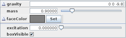
The build() method calls super.build() to perform all the model creation required by the super class, and then adds an additional widget for the boxVisible property to the control panel.
To run this example in ArtiSynth, select All demos > tutorial > SimpleMuscleWithProperties from the Models menu. The control panel will now contain an additional widget for the property boxVisible as shown in Figure 5.5. Toggling this property will make the box visible or invisible in the viewer.
5.3 Controllers and monitors
Application models can define custom controllers and monitors to control input values and monitor output values as a simulation progresses. Controllers are called every time step immediately before the advance() method, and monitors are called immediately after (Section 1.2.1). An example of controller usage is provided by ArtiSynth’s inverse modeling feature, which uses an internal controller to estimate the actuation signals required to follow a specified motion trajectory.
More precise details about controllers and monitors and how they interact with model advancement are given in the “Advancing Models in Time” section of the ArtiSynth Reference Manual.
5.3.1 Implementation
Applications may declare whatever controllers or monitors they require and then add them to the root model using the methods addController() and addMonitor(). They can be any type of ModelComponent that implements the Controller or Monitor interfaces. For convenience, most applications simply subclass the default implementations ControllerBase or MonitorBase and then override the necessary methods.
The primary methods associated with both controllers and monitors are:
apply(t0, t1) is the “business” method and is called once per
time step, with t0 and t1 indicating the start and end
times ![]() and
and ![]() associated with the step. initialize(t0)
is called whenever an application model’s state is set (or reset) at a
particular time
associated with the step. initialize(t0)
is called whenever an application model’s state is set (or reset) at a
particular time ![]() . This occurs when a simulation is first started
or after it is reset (with
. This occurs when a simulation is first started
or after it is reset (with ![]() ), and also when the state is
reset at a waypoint or during adaptive stepping.
), and also when the state is
reset at a waypoint or during adaptive stepping.
isActive() controls whether a controller or monitor is active; if isActive() returns false then the apply() method will not be called. The default implementations ControllerBase and MonitorBase, via their superclass ModelAgentBase, also provide a setActive() method to control this setting, and export it as the property active. This allows controller and monitor activity to be controlled at run time.
To enable or disable a controller or monitor at run time, locate it in the navigation panel (under the RootModel’s controllers or monitors list), chose Edit properties ... from the right-click context menu, and set the active property as desired.
Controllers and monitors may be associated with a particular model (among the list of models owned by the root model). This model may be set or queried using
If associated with a model, apply() will be called immediately before (for controllers) or after (for monitors) the model’s advance() method. If not associated with a model, then apply() will be called before or after the advance of all the models owned by the root model.
Controllers and monitors may also contain state, in which case they should implement the relevant methods from the HasState interface.
Typical actions for a controller include setting input forces or excitation values on components, or specifying the motion trajectory of parametric components (Section 1.2.4). Typical actions for a monitor include observing or recording the motion profiles or constraint forces that arise from the simulation.
5.3.1.1 Target positions and velocities
When setting the position and/or velocity of a dynamic component that has been set to be parametric (Section 1.2.4), a controller can opt to set its position and/or velocity directly. However, it is often preferable to instead set the component’s target position and/or target velocity, since this allows the solver to properly interpolate the position and velocity during the time step.
Whereas setting a position has no effect on velocity and vice versa, setting target positions and velocities does account for the coupling between the two. Specifically,
-
•
If a target position is set and the target velocity is not set, then during simulation the component’s position will be set to the target position and its velocity will be determined by differentiating the target position (albeit with a one-step time lag).
-
•
If a target velocity is set and the target position is not set, then during simulation the component’s velocity will be set to the target velocity and its position will be set by integrating the target velocity.
-
•
If both target position and target velocity are set (which is not commonly done), then during simulation both with be used to update the component’s position and velocity.
For Point-based components, target positions and velocities are exported as the properties targetPosition and targetVelocity, with the accessors:
For Frame-based components, target positions and velocities are exported as the properties targetPosition, targetOrientation and targetVelocity, with the accessors:
5.3.2 Example: A controller to move a point
A model showing an application-defined controller is defined in
artisynth.demos.tutorial.SimpleMuscleWithController
This simply extends SimpleMuscle (Section 4.5.2) and adds a controller which moves the fixed particle p1 along a circular path. The complete class definition is shown below:
A controller called PointMover is defined by extending ControllerBase and overriding the apply() method. It stores the
point to be moved in myPnt, and the initial position in
myPos0. The apply() method computes a target position for
the point that starts at myPos0 and then moves in a circle in the
![]() -
-![]() plane with an angular velocity of
plane with an angular velocity of ![]() rad/sec (lines 22-28).
rad/sec (lines 22-28).
The build() method calls super.build() to create the model used by SimpleMuscle, and then creates an instance of PointMover to move particle p1 and adds it to the root model (line 34). The viewer bounds are updated to make the circular motion more visible (line 36).
To run this example in ArtiSynth, select All demos > tutorial >
SimpleMuscleWithController from the Models menu. When
the model is run, the fixed particle p1 will trace
out a circular path in the ![]() -
-![]() plane.
plane.
5.4 Probes
In addition to controllers and monitors, applications can also attach streams of data, known as probes, to input and output values associated with the simulation. Probes derive from the same base class ModelAgentBase as controllers and monitors, but differ in that
-
1.
They are associated with an explicit time interval during which they are applied;
-
2.
They can have an attached file for supplying input data or recording output data;
-
3.
They are displayable in the ArtiSynth timeline panel.
A probe is applied (by calling its apply() method) only for time steps that fall within its time interval. This interval can be set and queried using the following methods:
The probe’s attached file can be set and queried using:
where filePath is a string giving the file’s path name. If filePath is relative (i.e., it does not start at the file system root), then it is assumed to be relative to the ArtiSynth working folder, which can be queried and set using the methods
of ArtisynthPath. The working folder can also be set from the ArtiSynth GUI by choosing File > Set working folder ....
If not explicitly set within the application, the working folder will default to a system dependent setting, which may be the user’s home folder, or the working folder of the process used to launch Artisynth.
Details about the timeline display can be found in the section “The Timeline” in the ArtiSynth User Interface Guide.
There are two types of probe: input probes, which are applied at the beginning of each simulation step before the controllers, and output probes, which are applied at the end of the step after the monitors. This is described in Section 1.2.1, and in even further detail in the “Advancing Models in Time” section of the ArtiSynth Reference Manual.
While applications are free to construct any type of probe by subclassing either InputProbe or OutputProbe, most applications utilize either NumericInputProbe or NumericOutputProbe, which explicitly implement streams of numeric data which are connected to properties of various model components. The remainder of this section will focus on numeric probes.
As with controllers and monitors, probes also implement a isActive() method that indicates whether or not the probe is active. Probes that are not active are not invoked. Probes also provide a setActive() method to control this setting, and export it as the property active. This allows probe activity to be controlled at run time.
To enable or disable a probe at run time, locate it in the navigation panel (under the RootModel’s inputProbes or outputProbes list), chose Edit properties ... from the right-click context menu, and set the active property as desired.
Probes can also be enabled or disabled in the timeline, by either selecting the probe and invoking activate or deactivate from the right-click context menu, or by clicking the track mute button (which activates or deactivates all probes on that track).
5.4.1 Numeric probe structure
Numeric probes are associated with:
-
•
A vector of temporally-interpolated numeric data;
-
•
One or more properties to which the probe is bound and which are either set by the numeric data (input probes), or used to set the numeric data (output probes).
The numeric data is implemented internally by a
NumericList, which stores the data
as a series of vector-valued knot points at prescribed times ![]() and
then interpolates the data for an arbitrary time
and
then interpolates the data for an arbitrary time ![]() using an
interpolation scheme provided by
Interpolation.
using an
interpolation scheme provided by
Interpolation.
Some of the numeric probe methods associated with the interpolated data include:
Interpolation schemes are described by the enumerated type Interpolation.Order and presently include:
- Step
-
Values at time
 are set to the values of the closest knot point
 such that
  .
. - Linear
-
Values at time
are set by linear interpolation of the knot points
 such that
  .
. - Parabolic
-
Values at time
are set by quadratic interpolation of the knots
 such that .
 - Cubic
-
Values at time
are set by cubic Catmull interpolation of the knots
 such that .
Each property bound to a numeric probe must have a value that can be mapped onto a scalar or vector value. Such properties are know as numeric properties, and whether or not a value is numeric can be tested usingNumericConverter.isNumeric(value).
By default, the total number of scalar and vector values associated with all the properties should equal the size of the interpolated vector (as returned by getVsize()). However, it is possible to establish more complex mappings between the property values and the interpolated vector. These mappings are beyond the scope of this document, but are discussed in the sections “General input probes” and “General output probes” of the ArtiSynth User Interface Guide.
5.4.2 Creating probes in code
This section discusses how to create numeric probes in code. They can also be created and added to a model graphically, as described in the section “Adding and Editing Numeric Probes” in the ArtiSynth User Interface Guide.
Numeric probes have a number of constructors and methods that make it relatively easy to create instances of them in code. For NumericInputProbe, there is the constructor
which creates a NumericInputProbe, binds it to a property located relative to the component c by propPath, and then attaches it to the file indicated by filePath and loads data from this file (see Section 5.4.4). The probe’s start and stop times are specified in the file, and its vector size is set to match the size of the scalar or vector value associated with the property.
To create a probe attached to multiple properties, one may use the constructor
which binds the probe to multiple properties specified relative to c by propPaths. The probe’s vector size is set to the sum of the sizes of the scalar or vector values associated with these properties.
For NumericOutputProbe, one may use the constructor
which creates a NumericOutputProbe, binds it to the property propPath located relative to c, and then attaches it to the file indicated by filePath. The argument interval indicates the update interval associated with the probe, in seconds; a value of 0.01 means that data will be added to the probe every 0.01 seconds. If interval is specified as -1, then the update interval will default to the simulation step size. This interval can also be accessed after the probe is created using
To create an output probe attached to multiple properties, one may use the constructor
As the simulation proceeds, an output probe will accumulate data, but this data will not be saved to any attached file until the probe’s save() method is called. This can be requested in the GUI for all probes by clicking on the Save button in the timeline toolbar, or for specific probes by selecting them in the navigation panel (or the timeline) and then choosing Save data in the right-click context menu.
Output probes created with the above constructors have a default interval of [0, 1]. A different interval may be set using setInterval(), setStartTime(), or setStopTime().
5.4.3 Example: probes connected to SimpleMuscle
A model showing a simple application of probes is defined in
artisynth.demos.tutorial.SimpleMuscleWithProbes
This extends SimpleMuscle (Section 4.5.2) to add an input probe to move particle p1 along a defined path, along with an output probe to record the velocity of the frame marker. The complete class definition is shown below:
The input and output probes are added using the custom methods createInputProbe() and createOutputProbe(). At line 14, createInputProbe() creates a new input probe bound to the targetPosition property for the component particles/p1 located relative to the MechModel mech. The same constructor attaches the probe to the filesimpleMuscleP1Pos.txt, which is read to load the probe data. The format of this and other probe data files is described in Section 5.4.4. The method PathFinder.getSourceRelativePath() is used to locate the file relative to the source directory for the application model (see Section 2.6). The probe is then given the name "Particle Position" (line 18) and added to the root model (line 19).
Similarly, createOutputProbe() creates a new output probe which is bound to the velocity property for the component frameMarkers/0 located relative to mech, is attached to the file simpleMuscleMkrVel.txt located in the application model source directory, and is assigned an update interval of 0.01 seconds. This probe is then named "FrameMarker Velocity" and added to the root model.
The build() method calls super.build() to create everything required for SimpleMuscle, calls createInputProbe() and createOutputProbe() to add the probes, and adjusts the MechModel viewer bounds to make the resulting probe motion more visible.
To run this example in ArtiSynth, select All demos > tutorial > SimpleMuscleWithProbes from the Models menu. After the model is loaded, the input and output probes should appear on the timeline (Figure 5.6). Expanding the probes should display their numeric contents, with the knot points for the input probe clearly visible. Running the model will cause particle p1 to trace the trajectory specified by the input probe, while the velocity of the marker is recorded in the output probe. Figure 5.7 shows an expanded view of both probes after the simulation has run for about six seconds.
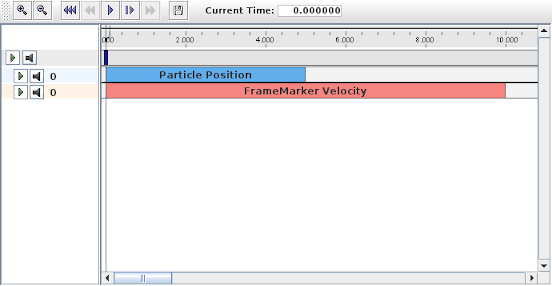
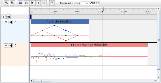
5.4.4 Data file format
The data files associated with numeric probes are ASCII files containing two lines of header information followed by a set of knot points, one per line, defining the numeric data. The time value (relative to the probe’s start time) for each knot point can be specified explicitly at the start of the each line, in which case the file takes the following format:
Knot point information begins on line 3, with each line being a
sequence of numbers giving the knot’s time followed by ![]() values,
where
values,
where ![]() is the vector size of the probe (i.e., the value returned by
getVsize()).
is the vector size of the probe (i.e., the value returned by
getVsize()).
Alternatively, time values can be implicitly specified starting at 0 (relative to the probe’s start time) and incrementing by a uniform timeStep, in which case the file assumes a second format:
For both formats, startTime, startTime, and scale are numbers giving the probe’s start and stop time in seconds and scale gives the scale factor (which is typically 1.0). interpolation is a word describing how the data should be interpolated between knot points and is the string value of Interpolation.Order as described in Section 5.4.1 (and which is typically Linear, Parabolic, or Cubic). vsize is an integer giving the probe’s vector size.
The last entry on the second line is either a number specifying a (uniform) time step for the knot points, in which case the file assumes the second format, or the keyword explicit, in which case the file assumes the first format.
As an example, the file used to specify data for the input probe in the example of Section 5.4.3 looks like the following:
Since the data is uniformly spaced beginning at 0, it would also be possible to specify this using the second file format:
5.4.5 Adding input probe data in code
It is also possible to specify input probe data directly in code, instead of reading it from a file. For this, one would use the constructor
which creates a NumericInputProbe with the specified property and with start and stop times indicated by t0 and t1. Data can then be added to this probe using the method
where data is an array of knot point data. This contains the
same knot point information as provided by a file (Section
5.4.4), arranged in row-major order. Times values
for the knots are either implicitly specified, starting at 0 (relative
to the probe’s start time) and increasing uniformly by the amount
specified by timeStep, or are explicitly specified at the
beginning of each knot if timeStep is set to the built-in
constant NumericInputProbe.EXPLICIT_TIME. The size of the data array should then be either ![]() (implicit time values) or
(implicit time values) or
![]() (explicit time values), where
(explicit time values), where ![]() is the probe’s vector size
and
is the probe’s vector size
and ![]() is the number of knots.
is the number of knots.
As an example, the data for the input probe in Section 5.4.3 could have been specified using the following code:
When specifying data in code, the interpolation defaults to Linear unless explicitly specified usingsetInterpolationOrder(), as in, for example:
Data can also be added incrementally, using the method
which adds a data knot the specified values at time t; values should have a size equal to the probe’s vector size. For example, the array-based example above could instead by implemented as
When an input probe is created without data specified in its constructor (e.g., by means of a probe data file), then it automatically adds knot points at its start and end times, with values set from the current values of its bound properties. Applying such a probe, without adding additional data, will thus leave the values of its properties unchanged.
The addData() methods described above do not remove existing knot points (although they will overwrite knots that exist at the same times). In order to replace all data, one can first call the method
which removes all knot points. Probes with no knots assign 0 to all their property values. Data can subsequently be added using the addData() methods. Alternatively, one can call
which behaves identically to the addData(double[],timeStep) method except that it first removes all existing data.
5.4.5.1 Extending data to the start and end
By explicitly using the clearData() or setData() methods, it is possible to create an input probe for which data is missing at its start and/or stop times. The behavior in that case is determined by the probe’s extendData property: if the property is set to true, then data values between the start time and the first knot, or the last knot and the stop time, are set to the values of the first and last knot, respectively. Otherwise, these data values are set to zero.
As with all properties, extendData can be set and queried in code using the accessors
The default value of extendData is true. As mentioned above, probes with no data set their data values uniformly to 0.
5.4.6 Setting data from text or CSV files and other probes
Applications can import/export data from/to text and CSV files. For both
formats, the file is assumed to contain one line per time value, with numbers
separated by either whitespace (for text) or a comma character (for CSV). Time
values may or may not be included; if ![]() is the probe’s vector size, each line
will have
is the probe’s vector size, each line
will have ![]() values in the former case and
values in the former case and ![]() in the latter. As an
example, a text file including time values for a probe with
in the latter. As an
example, a text file including time values for a probe with ![]() and four
time values might look like
and four
time values might look like
while an equivalent CSV file could look like
Importing and exporting can be done by the following methods:
| void importTextData (File file, double timeStep) |
Import from a text file. |
| void exportTextData (File file) |
Export to a text file. |
| void exportTextData (File file, String fmtStr, boolean includeTime) |
Export to a text file. |
| void importCsvData (File file, double timeStep) |
Import from a CSV file. |
| void exportCsvData (File file) |
Export to a CSV file. |
| void exportCsvData (File file, String fmtStr, boolean includeTime) |
Export to a CSV file. |
| void importData (File file, double timeStep) |
Infer text or CSV from file suffix. |
The timeStep argument to the import methods indicates whether the file
includes time values: if it is ![]() , time values should be included;
otherwise, time values are computed from k*timeStep, where k is the
the line number starting at 0. The arguments fmtStr and includeTime
for some of the export methods specify a C-style numeric format string
(see NumberFormat) and whether or not time values
should be included; the defaults are "%g" (full general precision) and
true.
, time values should be included;
otherwise, time values are computed from k*timeStep, where k is the
the line number starting at 0. The arguments fmtStr and includeTime
for some of the export methods specify a C-style numeric format string
(see NumberFormat) and whether or not time values
should be included; the defaults are "%g" (full general precision) and
true.
It is also possible to copy data from one probe to another, using the method
| void setData (NumericProbeBase src, boolean useAbsoluteTime) |
All knot points and values are copied from src, which can be any numeric probe (input or output), with the only restriction being that its vector size must equal or exceed that of the calling probe (extra values are ignored). If useAbsoluteTime is true, time values are mapped between the probes using absolute time; otherwise, probe relative time is used. When using this method, care should be taken to ensure that the there will be knot points to cover the start and stop times of the calling probe.
5.4.7 Tracing probes
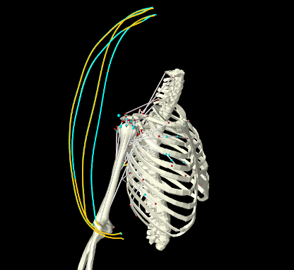
It is often useful to follow the path or evolution of a position or vector quantity as it evolves in time during a simulation. For example, one may wish to trace out the path of some points, as per Figure 5.8, which traces the actual and desired paths of some marker points during an inverse simulation of the type described in Chapter 10.
ArtiSynth supplies TracingProbes that can be used for this purpose. A tracing probe can be attached to any component that implements the interface Traceable, for any of the properties that are exported by its getTraceables() method. At present, Traceable is implemented for the following components:
Tracing probes are easily created using the RootModel method
| TracingProbe addTracingProbe (Traceable comp, String propName, double startTime, double stopTime) |
which produces a tracing probe of specified duration for the indicated component and property name pair. During simulation, the probe will record the desired property at the rate defined by its updateInterval, and also render it in the viewer. In cases where the probe renders all its stored values (as with PointTracingProbes, described below), the interval at which this occurs can be controlled by its renderInterval property, accessed in code via
| double getRenderInterval() |
Return the render interval |
| void setRenderInterval(double interval) |
Set the render interval (seconds) |
Specifying a render interval of -1 (the default) will cause the render interval to equal the update interval.
Two types of tracing probes are currently implemented:
- PointTracingProbe
-
Created for point properties, this renders the path of the point position over the duration of the probe, either as a continuous curve (if the probe’s pointTracing property is false, the default setting), or as discrete points. The appearance of the rendering is controlled by subproperties of the probe’s render properties, using lineStyle, lineRadius, lineWidth and lineColor (for continuous curves) or pointStyle, pointRadius, pointSize and pointColor (for points).
- VectorTracingProbe
-
Created for vector properties, this renders the vector quantity at the current simulation time as a line segment anchored at the current position of the component. The length of the line segment is controlled by the probe’s lengthScaling property, and other aspects of the appearance are controlled by the subproperties lineStyle, lineRadius, lineWidth and lineColor of the probe’s render properties. Vector tracing is mostly used to visualize instantaneous forces.
The following code fragment attaches a tracing probe to the last frame marker of the MultiJointedArm example of Section 3.5.16:
with the results shown in Figure 5.9 (left). To instead render the output as points, and with a coarser render interval of 0.02, one could modify the probe properties using
with the results shown in Figure 5.9 (right).

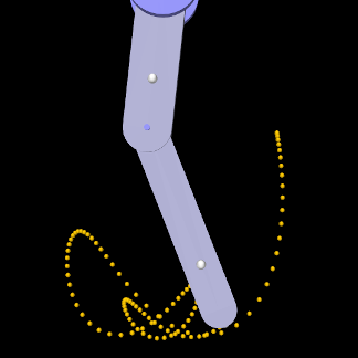
|
Tracing probes can also be created and edited interactively, as described in the section “Point Tracing” of the ArtiSynth User Interface Guide.
5.4.8 Position probes
Applications often find it useful to parametrically control the position of point or frame-based components, which include Point, Frame, FixedMeshBody, and their subclasses (e.g., Particle, RigidBody, and FemNode3d). This can be done by setting either the components’ position or targetPosition properties, and (for frame-based components) their orientation or targetOrientation properties. As described in Section 5.3.1.1, setting targetPosition and targetOrientation is often preferable as this will automatically update the component’s velocity, and so provide more information to the integrator, whereas setting position and orientation will leave the velocity unchanged.
When controlling the position and/or velocity of dynamic components, which include Point and Frame, it is important to ensure that their dynamic property is set to false and that they are unattached. Otherwise, the dynamic simulation will override any attempt at setting their position or velocity.
For frame-based components, the orientation and targetOrientation
properties describe their spatial orientation using an instance of
AxisAngle, which represents
a single rotation ![]() about a specific axis
about a specific axis ![]() in world coordinates (any
3D rotation can be expressed this way). However, when using this in a probe to
control or observe a frame-based component’s pose over time, a couple
of issues arise:
in world coordinates (any
3D rotation can be expressed this way). However, when using this in a probe to
control or observe a frame-based component’s pose over time, a couple
of issues arise:
-
•
There are other rotation representations that may be more useful or easier to specify, such as z-y-x or x-y-z rotations, in either radians or degrees.
-
•
Whatever rotation representation is used, care must be taken when interpolating it between knot points. Rotations cannot be treated as vectors and interpolation must instead take the form of curves on the 3D rotation group
 . The details are beyond the scope of this document but
were initially described by Shoemake [23].
. The details are beyond the scope of this document but
were initially described by Shoemake [23].
To address these issues, ArtiSynth supplies PositionInputProbe and PositionOutputProbe, which can be used to control or observe the position of one or more points or frame-based components, while offering a variety of rotation representations and handling rotation interpolation correctly. In particular, PositionInputProbes allow an application to supply key-frame animation control poses for frame-based components.
PositionInputProbes can be created with the constructors
In the above, name is the probe name (optional, can be null), and comp and comps refer to the component(s) to be assigned to the probe; as indicated above, these must be instances of Point, Frame, or FixedMeshBody. rotRep is an instance of RotationRep, which indicates how rotations should be represented, as described further below. The argument useTargetProps, if true, specifies that the probe should be attached to the targetPosition and (for frames) targetOrientation properties, vs. the position and orientation properties (if false). startTime and stopTime give the probe’s start and stop times, while filePath specifies a probe file from which to read in the probe’s basic parameters and data, per Section 5.4.4. Probes constructed without a file need to have data added, as per Section 5.4.5.
As indicated by the constructors, PositionInputProbes can control multiple
point and frame-based components, and this arrangement affects the size and
composition of the data vector. Each point component requires 3 numbers
specifying position, while each frame component requires ![]() numbers
specifying position and orientation, where
numbers
specifying position and orientation, where ![]() is the size of the
rotation representation. Although the orientation and targetOrientation properties describe rotation using an
AxisAngle, this will be converted
into knot point data based on the assigned RotationRep, with
is the size of the
rotation representation. Although the orientation and targetOrientation properties describe rotation using an
AxisAngle, this will be converted
into knot point data based on the assigned RotationRep, with ![]() equal to
either 3 or 4. The total size
equal to
either 3 or 4. The total size ![]() of the data vector is then
of the data vector is then
where ![]() is the number of points and
is the number of points and ![]() is the number of frames.
is the number of frames.
RotationRep provides a variety of ways to specify the rotation and applications can choose the most suitable:
- ZYX
-
Successive rotations, in radians, about the
 axes;
axes;  .
. - ZYX_DEG
-
Successive rotations, in degrees, about the
axes; . - XYZ
-
Successive rotations, in radians, about the
 axes; .
 - XYZ_DEG
-
Successive rotations, in degrees, about the
axes; . - AXIS_ANGLE
-
Axis-angle representation (
 , ), with the given in
radians;
, ), with the given in
radians;  . The axis does not need to be normalized.
 - AXIS_ANGLE_DEG
-
Axis-angle representation (
, ), with the given in
degrees; . The axis does not need to be normalized. - QUATERNION
-
Unit quaternion;
.
As a possibly more convenient alternative to the methods of Section 5.4.5, and to avoid having to explicitly pack the position and orientation information into the probe’s knot data, PositionInputProbes also supply the following methods to set the knot data for individual components being controlled by the probe:
| setPointData (Point point, double time, Vector3d pos) |
Set point position at a given time. |
| setFrameData (ModelComponent frame, double time, RigidTransform3d TFW) |
Set frame position/orientation at a given time. |
Each of these methods writes only the portion of the knot point at the indicated time that corresponds to the specified component; other portions are left unchanged or initialized to 0. For frames, TFW gives the pose (position/orientation) in the form of the transform from frame to world coordinates, and the orientation is transformed into knot point data according to the probe’s rotation representation.
PositionOutputProbes can be created with constructors analogous to PositionInputProbe:
The knot data format is the same as for PositionInputProbes, with rotations represented according to the setting of rotRep. There is no useTargetProps argument because PositionOutputProbes bind only to the position and orientation properties. If present, the filePath and interval arguments specify an attached file name for saving probe data and the update interval in seconds. Setting interval to -1 causes updating to occur at the simulation update rate, and this is the default for constructors without an interval argument.
5.4.9 Velocity probes
As with positions, applications may sometimes need to parametrically control or observe the velocity of point or frame-based components, which include Point, Frame, and their subclasses (but not FixedMeshBody, as this is not a dynamic component and so does not maintain a velocity). This can be done by setting either the components’ velocity or targetVelocity properties, with the latter sometimes preferable as it will automatically update the component’s position, whereas setting velocity will not. For frame-based components, velocity and targetVelocity are described by a 6-DOF Twist component that contains both translational and angular velocities. Unlike with finite rotations, there is only one representation for angular velocity (as a vector with units of radians/sec) and there are no interpolation issues.
When the position of a component is being controlled it is typically not necessary to also supply velocity information. This is especially true for position probes bound to targetPosition and targetOrientation properties, since these update velocity information automatically. However, for position probes bound to position and orientation, it can be sometimes be useful to use a velocity probe to also supply velocities. One example of this is when components are being tracked by inverse simulation (Chapter 10), as this extra information this can reduce tracking error and lag.
ArtiSynth provides VelocityInputProbe and VelocityOutputProbe to control or monitor the velocities of one or more point or frame-based components. The constructors for these are:
For all of these, the arguments are completely analogous to those for the constructors of PositionInputProbe and PositionOutputProbe, with the argument rotRep absent because it is not needed, and with useTargetProps specifying whether the probe should be attached to the targetVelocity or velocity properties.
If a position probe (either input or output) exists for a given collection of components, it is possible to automatically create a VelocityInputProbe for the same set of components, using one of the following static methods:
| VelocityInputProbe VelocityInputProbe.createNumeric (String name, NumericProbeBase source, double interval) |
Create by numeric differentiation. |
| VelocityInputProbe VelocityInputProbe.createInterpolated (String name, NumericProbeBase source, double interval) |
Create by interpolation. |
Both take an optional probe name and source probe. The update interval gives the time interval between the created knot points, with -1 causing this to be taken from the source. The first method creates the probe by numeric differentiation of the source’s position data and should be used only when the source’s data is dense, while the second method finds the derivative from the interpolation method of the source probe (as described by getInterpolationOrder()) and is better suited when the source data is sparse (although the resulting velocity will not be continuous unless the interpolation order is greater than linear).
The following code fragments creates a position probe and then uses this to generate a velocity probe:
5.4.10 Example: controlling a point and frame
 |
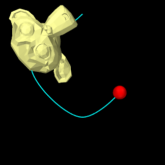 |
A model demonstrating position and velocity probes is defined in
artisynth.demos.tutorial.PositionProbes
It creates a point and a rigid body (using the Blender monkey mesh), sets both to be non-dynamic, uses position and velocity probes to control their positions, and uses PositionOutputProbe and VelocityOutputProbe to monitor the resulting positions and velocities. The model class definition, excluding the import directives, is shown here:
The build() creates a MechModel and then adds to it a rigid body (created from the Blender monkey mesh) and a particle (lines 8-19). Both components are made non-dynamic to allow their positions and velocities to be controlled, and references to them are placed in a list used to create the probes (lines 21-24).
A PositionInputProbe for controlling the positions is created at lines 26-44, using a rotation representation of RotationRep.ZYX (successive rotations about the z-y-x axes, in radians). For this example, the useTargetProps is set to false (so that the probe binds to position and orientation), because we are going to be specifying velocities explicitly using another probe. Data for the probe is set using setData(), with the point and monkey positions/poses specified, in order, for times 0, 0.5, 1.0, 1.5 and 2. As per the rotation specification, poses for the monkey are given by 3 positions and 3 z-y-x rotations. Because the data is sparse, the probe’s interpolation order is set to Cubic to generate smooth motions.
A VelocityInputProbe is created by differentiating the position probe (lines 47-49); createInterpolated() is used because the position data is sparse and so numeric differentiation would yield bad results.
Finally, output probes to track both the resulting positions and velocities, together with a tracing probe to render the point’s path in cyan, are created at lines 51-65. When creating the PositionOutputProbe, we use the same rotation representation RotationRep.ZYX as for the input probe, but this is not necessary. For example, if one were to instead specify RotationRep.QUATERNION, then the frame orientations would be specified as quaternions.
To run this example in ArtiSynth, select All demos > tutorial > PositionProbes from the Models menu. When run, both the point and monkey will orbit around each other, with the point path being displayed by the tracing probe (Figure 5.10, right).
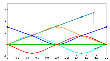 |
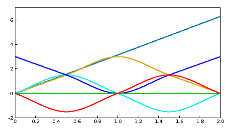 |
Several things about this demo should be noted:
-
•
The use of setData() in creating the position probe could be replaced by setPointData() and setFrameData(), as per
pip.setPointData (point, 0.5, new Point3d(-1.5,0,1.5));pip.setPointData (point, 1.0, new Point3d(0,0,0));pip.setPointData (point, 1.5, new Point3d(1.5,0,1.5));pip.setFrameData (monkey, 0.5, new RigidTransform3d(1.5,0,1.5, 0,PI/2,0));pip.setFrameData (monkey, 1.0, new RigidTransform3d(0.0,0,3.0, 0,PI,0));pip.setFrameData (monkey, 1.5, new RigidTransform3d(-1.5,0,1.5, 0,3*PI/2,0));Here, we can omit data for times 0 and 2 (at the probe’s start and end) because the motion begins and ends at the components’ initial positions, for which data was automatically added when the probe was created. (Likewise, data for times 0 and 2 could be omitted in the original code if addData() was used instead of setData()).
-
•
Position probes handle angle wrapping correctly. In the position input probe, the y-axis rotation for the monkey goes from
 to between
  and
and  . However, by generating
“minimal distance” motions, interpolation proceeds as though the final angle
was specified as
. However, by generating
“minimal distance” motions, interpolation proceeds as though the final angle
was specified as  , allowing the circular motion to complete instead of
backtracking (although in the display plot, there is an apparent discontinuity
at
, allowing the circular motion to complete instead of
backtracking (although in the display plot, there is an apparent discontinuity
at  ; see Figure 5.11, left). Likewise, in
position output probes, as data is added, the rotation representation is
chosen to be as near as possible to the previous, so that in the
example the recorded rotation does indeed arrive at instead of
(Figure 5.11, right).
; see Figure 5.11, left). Likewise, in
position output probes, as data is added, the rotation representation is
chosen to be as near as possible to the previous, so that in the
example the recorded rotation does indeed arrive at instead of
(Figure 5.11, right). -
•
Since useTargetProps is set to false in the example, the velocity input probe is needed to set the component velocities; if this probe is made inactive (either in code or interactively in the timeline), then while the bodies will still move, no velocities will be set and the data in the velocity output probe will be uniformly 0.
Alternatively, if useTargetProps is set to true, then the input probes will be bound to targetPosition, targetOrientation, and targetVelocity, and both positions and velocities will be set for the components if either input probe is active. Reflecting the description in Section 5.3.1.1:
-
–
If the position input probe is active and the velocity input probe is inactive, then the velocities will be determined by differentiating the target position inputs (albeit with a one-step time lag).
-
–
If the position input probe is inactive and the velocity input probe is active, then the positions will be determined by integrating the target velocity inputs. Note that in this case, when the probes terminate, the components will continue moving with their last specified velocity.
-
–
If both the position and velocity input probes are active, then both the target position and velocity information will be used to update the component positions and velocities.
This provides a useful example of how target properties work.
-
–
5.4.11 Numeric monitor probes
In some cases, it may be useful for an application to deploy an output probe in which the data, instead of being collected from various component properties, is generated by a function within the probe itself. This ability is provided by a NumericMonitorProbe, which generates data using its generateData(vec,t,trel) method. This evaluates a vector-valued function of time at either the absolute time t or the probe-relative time trel and stores the result in the vector vec, whose size equals the vector size of the probe (as returned by getVsize()). The probe-relative time trel is determined by
| (5.0) |
where tstart and scale are the probe’s start time and scale factors as returned by getStartTime() and getScale().
As described further below, applications have several ways to control how a NumericMonitorProbe creates data:
-
•
Provide the probe with a DataFunction using the setDataFunction(func) method;
-
•
Override the generateData(vec,t,trel) method;
-
•
Override the apply(t) method.
The application is free to generate data in any desired way, and so in this sense a NumericMonitorProbe can be used similarly to a Monitor, with one of the main differences being that the data generated by a NumericMonitorProbe can be automatically displayed in the ArtiSynth GUI or written to a file.
The DataFunction interface declares an eval() method,
void eval (VectorNd vec, double t, double trel)
that for NumericMonitorProbes evaluates a vector-valued function of time, where the arguments take the same role as for the monitor’s generateData() method. Applications can declare an appropriate DataFunction and set or query it within the probe using the methods
The default implementation generateData() checks to see if a data function has been specified, and if so, uses that to generate the probe data. Otherwise, if the probe’s data function is null, the data is simply set to zero.
To create a NumericMonitorProbe using a supplied DataFunction, an application will create a generic probe instance, using one of its constructors such as
and then define and instantiate a DataFunction and pass it to the probe using setDataFunction(). It is not necessary to supply a file name (i.e., filePath can be null), but if one is provided, then the probe’s data can be saved to that file.
A complete example of this is defined in
artisynth.demos.tutorial.SinCosMonitorProbe
the listing for which is:
In this example, the DataFunction is implemented using the class SinCosFunction, which also implements Clonable and the associated clone() method. This means that the resulting probe will also be duplicatable within the GUI. Alternatively, one could implement SinCosFunction by extending DataFunctionBase, which implements Clonable by default. Probes containing DataFunctions which are not Clonable will not be duplicatable.
When the example is run, the resulting probe output is shown in the timeline image of Figure 5.12.
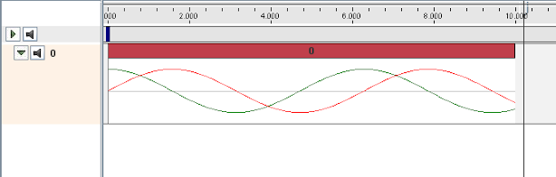
As an alternative to supplying a DataFunction to a generic NumericMonitorProbe, an application can instead subclass NumericMonitorProbe and override either its generateData(vec,t,trel) or apply(t) methods. As an example of the former, one could create a subclass as follows:
Note that when subclassing, one must also create constructor(s) for that subclass. Also, NumericMonitorProbes which don’t have a DataFunction set are considered to be clonable by default, which means that the clone() method may also need to be overridden if cloning requires any special handling.
5.4.12 Numeric control probes
In other cases, it may be useful for an application to deploy an input probe which takes numeric data, and instead of using it to modify various component properties, instead calls an internal method to directly modify the simulation in any way desired. This ability is provided by a NumericControlProbe, which applies its numeric data using its applyData(vec,t,trel) method. This receives the numeric input data via the vector vec and uses it to modify the simulation for either the absolute time t or probe-relative time trel. The size of vec equals the vector size of the probe (as returned by getVsize()), and the probe-relative time trel is determined as described in Section 5.4.11.
A NumericControlProbe is the Controller equivalent of a NumericMonitorProbe, as described in Section 5.4.11. Applications have several ways to control how they apply their data:
-
•
Provide the probe with a DataFunction using the setDataFunction(func) method;
-
•
Override the applyData(vec,t,trel) method;
-
•
Override the apply(t) method.
The application is free to apply data in any desired way, and so in this sense a NumericControlProbe can be used similarly to a Controller, with one of the main differences being that the numeric data used can be automatically displayed in the ArtiSynth GUI or read from a file.
The DataFunction interface declares an eval() method,
void eval (VectorNd vec, double t, double trel)
that for NumericControlProbes applies the numeric data, where the arguments take the same role as for the monitor’s applyData() method. Applications can declare an appropriate DataFunction and set or query it within the probe using the methods
The default implementation applyData() checks to see if a data function has been specified, and if so, uses that to apply the probe data. Otherwise, if the probe’s data function is null, the data is simply ignored and the probe does nothing.
To create a NumericControlProbe using a supplied DataFunction, an application will create a generic probe instance, using one of its constructors such as
and then define and instantiate a DataFunction and pass it to the probe using setDataFunction(). The latter constructor creates the probe and reads in both the data and timing information from the specified file.
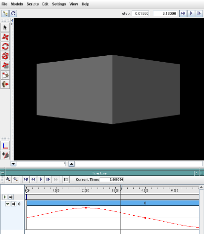
A complete example of this is defined in
artisynth.demos.tutorial.SpinControlProbe
the listing for which is:
This example creates a simple box and then uses a NumericControlProbe to spin it about the ![]() axis, using a DataFunction implementation called SpinFunction. A clone method
is also implemented to ensure that the probe will be duplicatable in
the GUI, as described in Section 5.4.11. A
single channel of data is used to control the orientation angle of the
box about
axis, using a DataFunction implementation called SpinFunction. A clone method
is also implemented to ensure that the probe will be duplicatable in
the GUI, as described in Section 5.4.11. A
single channel of data is used to control the orientation angle of the
box about ![]() , as shown in Figure 5.13.
, as shown in Figure 5.13.
Alternatively, an application can subclass NumericControlProbe and override either its applyData(vec,t,trel) or apply(t) methods, as described for NumericMonitorProbes (Section 5.4.11).
5.5 Working with TRC data
The TRC data format was originally developed by Motion Analysis Corporation to describe marker position data acquired during motion capture. An overview of the format is provided as part of the OpenSim documentation.
ArtiSynth supplies a simple reader and writer for TRC data, with the reader able to create probes directly from TRC files and the writer able to write files directly from probes.
It is assumed the TRC data is tab delimited; files that do not use tabs to separate their data will not be readable. There may also be other limitations of which we are unaware.
5.5.1 TRC reader
TRCReader allows one to read TRC data from a file using the simple code fragment
Another constructor also exists that accepts a string file name argument.
Both the constructors and the readData() method throw an IOException, which must either be handled in a try/catch block or thrown by the calling method.
Once the data has been read, it may be queried with the following methods:
| int numFrames() |
Return the number of frames. |
| double getFrameTime (int fidx) |
Return time of the fidx-th frame. |
| int numMarkers() |
Return the number of markers. |
| ArrayList<String> getMarkerLabels() |
Return all the marker labels. |
| int getMarkerIndex (String label) |
Return index of the labeled marker. |
| ArrayList<Point3d> getMarkerPositions (int fidx) |
Return all marker positions at frame fidx. |
| void getMarkerPositions (VectorNd mpos, int fidx) |
Return all marker positions at frame fidx into mpos. |
| Point3d getMarkerPosition (int fidx, int midx) |
Return position of midx-th marker at frame fidx. |
| Point3d getMarkerPosition (int fidx, String label) |
Return position of labeled marker at frame fidx. |
Both the frame and marker indices in the above methods are 0-based.
Once read, marker positions and frame times may be transformed, which may be useful for adjusting coordinate frames or units:
| void scaleMarkerPositions (double s) |
Scale marker positions by s. |
| void transformMarkerPositions (AffineTransform3dBase X) |
Apply the transform X to the marker positions. |
| void transformFrameTimes (double s, double b) |
Transform frame times |
TRCReader also supplies the following methods for creating PositionInputProbes directly from the data:
For these, name is the probe name (optional, can be null), points are the points to which the probe should be attached, useTargetProps indicates if the targetPosition or position properties should be bound, startTime and stopTime give the start and stop times, and labels, if present, gives a list of the marker labels that should be used for each point; otherwise, points are assigned to marker data in order.
As a convenience, the following static methods are also supplied:
These read the data directly from the supplied TRC file, assigning the probe a start time of 0 and a stop time determined from the last frame time.
5.5.2 TRC writer
TRCWriter allows an application to write a TRC file directly from the data in a numeric probe, using a code fragment such as
A constructor also exists that accepts a string file name argument.
The full signature for writeData() is
| void writeData (NumericProbeBase probe, List<String> labels) |
where probe is any type of probe associated with position or targetPosition properties for a set of Point components. The labels argument is an optional list of marker labels that should be assigned to the data for each point. If this is not supplied, labels are assigned automatically, either from the point names, or when these are null, by prepending "mkr" to the marker index.
The writeData() method throws an IOException, which must either be handled in a try/catch block or thrown by the calling method.
TRCWriter also supplies a few methods that can be used to format the data before it is written:
| String getNumberFormat() |
Return the format string for float data. |
| void setNumberFormat (String fmtStr) |
Set the format string for float data. |
| String getUnitsString() |
Return the string used to represent units. |
| void setUnitsString (String str) |
Set the string used to represent units. |
For convenience, the following static methods are also provided:
| void write (File file, NumericProbeBase probe, List<String> labels) | |
| void write (String fileName, NumericProbeBase probe, List<String> labels) | |
5.5.3 Example: moving MultiJointedArm with TRC data
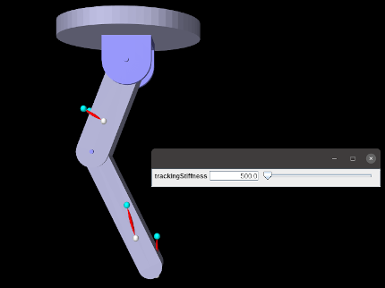
The example model
artisynth.demos.tutorial.TRCMultiJointedArm
illustrates several features that have been introduced in this chapter. It extends the model MultiJointedArm, previously described in Section 3.5.16. Then it reads TRC data defining target trajectories for the markers attached to the arm, with the intention of moving the arm. While a standard way to make marker data move an articulated structure is to employ an inverse kinematic solver (Section 10.5), this example uses a simpler solution. For each marker, a target point is defined and attached to it by means of a spring. The target points (which are non-dynamic) are then moved by means of a PositionInputProbe created from the TRC data. As they move, they drag the markers (and the attached bodies) around by means of the resulting spring forces. It can be shown that the resulting rest position of the system is identical to that of the inverse kinematic solver of Section 10.5.1 (assuming equal marker weights).
Tracking accuracy increases with spring stiffness (although very high stiffnesses may cause stability issues). To illustrate this relationship, a control panel is created that allows the user to adjust the spring stiffness interactively. To be able to control the stiffness of one spring with a single parameter, a custom model property, called trackingStiffness, is created per the description of Section 5.2, to control the stiffness values for all the springs.
The model’s class definition, excluding import directives, is given in
The first parts of the code define the trackingStiffness property, by first creating a local static property list (myProps) that inherits from the parent class MultiJointedArm.class (lines 9-10). A static block adds the property definition (lines 12-16), and the new list is made visible by a local implementation of getAllPropertyInfo() (lines 18-20). Get/set accessors are then defined for the property (lines 22-36). The property value is kept in the member variable myTrackingStiffness, but when it is set the stiffness is updated for all springs stored in the MechModel’s axial spring list.
The build() method starts by calling super.build() to create the original MultiJointedArm model (line 39), after which a reference to the created MechModel will be stored in the inherited member myMech. Then for each model marker, a target point is created, together with a connecting axial spring (lines 41-50). For simplicity, the targets and springs are stored in the MechModel’s default points and axialSprings lists, but they could be stored in custom containers, as per Section 4.8.
Next, TRC marker data is read from the file "data/multiJointMkrs.trc" located relative to the model’s source folder, using the TRCReader described in Section 5.5.1. This is used to create a PositionInputProbe attached to the target points (which are located under myMech.points()) (lines 57-60). Lastly, a control panel is created to allow adjustment of the tracking stiffness, and some render properties are set.
The last part of the class definition overrides the method postscanInitialize(), which is called in place of the build() method when a model is read from an ArtiSynth .art file. This method should initialize any class members which are unknown to the component hierarchy and would normally be set in the build() method. In this case, it is necessary to initialize myMech, which is needed by setTrackingStiffness() and would otherwise not be set. Models which are not intended to be saved to .art files do not need to override postscanInitialize().
To run this example in ArtiSynth, select All demos > tutorial > TRCMultiJointedArm from the Models menu. The demo will appear, together with the control panel (shown overlaid in Figure 5.14). When the model is run, the target points will be moved under the control of their position probe, dragging the markers along via the attached springs. Increasing/decreasing the spring stiffness will decrease/increase the tracking error.
5.6 Application-Defined Menu Items
Application models can define custom menu items that appear under the Application menu in the main ArtiSynth menu bar.
This can be done by implementing the interface HasMenuItems in either the RootModel or any of its top-level components (e.g., models, controllers, probes, etc.). The interface contains a single method
which, if the component has menu items to add, should append them to items and return true.
The RootModel and all models derived from ModelBase implement HasMenuItems by default, but with getMenuItems() returning false. Models wishing to add menu items should override this default declaration. Other component types, such as controllers, need to explicitly implement HasMenuItems.
Note: the Application menu will only appear if getMenuItems() returns true for either the RootModel or one or more of its top-level components.
getMenuItems() will be called each time the Application menu is selected, so the menu itself is created on demand and can be varied to suit the current system state. In general, it should return items that are capable of being displayed inside a Swing JMenu; other items will be ignored. The most typical item is a Swing JMenuItem. The convenience method createMenuItem(listener,text,toolTip) can be used to quickly create menu items, as in the following code segment:
This creates three menu items, each with this specified as an ActionListener and no tool-tip text, and appends them to items. They will then appear under the Application menu as shown in Figure 5.15.
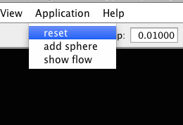
To actually execute the menu commands, the items returned by getMenuItems() need to be associated with an ActionListener (defined in java.awt.event), which supplies the method actionPerformed() which is called when the menu item is selected. Typically the ActionListener is the component implementing HasMenuItems, as was assumed in the example declaration of getMenuItems() shown above. RootModel and other models derived from ModelBase implement ActionListener by default, with an empty declaration of actionPerformed() that should be overridden as required. A declaration of actionPerformed() capable of handling the menu example above might look like this:
5.6.1 Smoothing probe data
Numeric probe data can also be smoothed, which is convenient for removing noise from either input or output data. Different smoothing methods are available; at the time of this writing, they include:
- Moving average
-
Applies a mean average filter across the knots, using a moving window whose size is specified by the window size field. The window is centered on each knot, and is reduced in size near the end knots to ensure a symmetric fit. The end knot values are not changed. The window size must be odd and the window size field enforces this.
- Savitzky Golay
-
Applies Savitzky-Golay smoothing across the knots, using a moving window of size
 . Savitzky-Golay smoothing works by fitting the
data values in the window to a polynomial of a specified degree
. Savitzky-Golay smoothing works by fitting the
data values in the window to a polynomial of a specified degree  , and
using this to recompute the value in the middle of the window. The
polynomial is also used to interpolate the first and last
, and
using this to recompute the value in the middle of the window. The
polynomial is also used to interpolate the first and last  values, since it is not possible to center the window on these.
The window size
and the polynomial degree are specified by the
window size and polynomial degree fields. must be odd,
and must also be larger than , and the fields enforce these
constraints.
These operations may be applied with the following numeric probe methods:
| void smoothWithMovingAverage (double winSize) |
Moving average smoothing over a specified window. |
| void smoothWithSavitzkyGolay ( double winSize, int deg) |
Savitzky Golay smoothing with specified window and degree. |
Chapter 6 Finite Element Models
This chapter details how to construct three-dimensional finite element models, and how to couple them with the other simulation components described in previous sections (e.g. particles and rigid bodies). Finite element muscles, which have additional properties that allow them to contract given activation signals, are discussed in Section 6.9. An example FEM model of the masseter, coupled to a rigid jaw and maxilla, is shown in Figure 6.1.
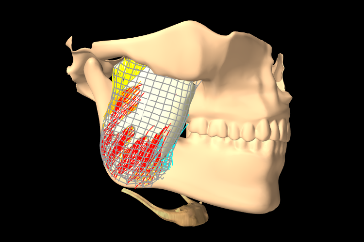
Most of the ArtiSynth components described here are contained in the packages
artisynth.core.modelbase artisynth.core.femmodels artisynth.core.materials
6.1 Overview
The finite element method (FEM) is a numerical technique used for solving a system of partial differential equations (PDEs) over some domain. The general approach is to divide the domain into a set of building blocks, referred to as elements. These partition the space, and form local domains over which the system of equations can be locally approximated. The corners of these elements, the nodes, become control points in a discretized system. The solution is then assumed to be smoothly interpolated across the elements based on values determined at the nodes. Using this discretization, the differential system is converted into an algebraic one, which is often linearized and solved iteratively.
In ArtiSynth, the PDEs considered are the governing equations of continuum mechanics: the conservation of mass, momentum, and energy. To complete the system, a constitutive equation is required that describes the stress-strain response of the material. This constitutive equation is what distinguishes between material types. The domain is the three-dimensional space that the model occupies. This must be divided into small elements which accurately represent the geometry. Within each element, the PDEs are sampled at a set of points, referred to as integration points, and terms are numerically integrated to form an algebraic system to solve.
The purpose of the rest of this chapter is to describe the construction and use of finite elements models within ArtiSynth. It does not further discuss the mathematical framework or theory. For an in-depth coverage of the nonlinear finite element method, as applied to continuum mechanics, the reader is referred to the textbook by Bonet and Wood [6].
6.1.1 FemModel3d
The basic type of finite element model is implemented in the class FemModel3d. This class controls some properties that are used by the model as a whole. The key ones that affect simulation dynamics are:
| Property | Description |
|---|---|
| density | The density of the model |
| material | An object that describes the material’s constitutive law (i.e. its stress-strain relationship). |
| particleDamping | Proportional damping associated with the particle-like motion of the FEM nodes. |
| stiffnessDamping | Proportional damping associated with the system’s stiffness term. |
These properties can be set and retrieved using the methods
| void setDensity (double density) |
Sets the density. |
| double getDensity() |
Gets the density. |
| void setMaterial (FemMaterial mat) |
Sets the FEM’s material. |
| FemMaterial getMaterial() |
Gets the FEM’s material. |
| void setParticleDamping (double d) |
Sets the particle (mass) damping. |
| double getParticleDamping() |
Gets the particle (mass) damping. |
| void setStiffnessDamping (double d) |
Sets the stiffness damping. |
| double getStiffnessDamping() |
Gets the stiffness damping. |
Keep in mind that ArtiSynth is essentially “unitless” (Section 4.2), so it is the responsibility of the developer to ensure that all properties are specified in a compatible way.
The density of the model is used to compute the mass distribution throughout the volume. Note that we use a diagonally lumped mass matrix (DLMM) formulation, so the mass is assumed to be concentrated at the location of the discretized FEM nodes. To allow for a spatially-varying density, densities can be explicitly set for individual elements, or masses can be explicitly set for individual nodes.
The FEM’s material property is a delegate object used to compute stress and stiffness within individual elements. It handles the constitutive component of the model, as described in more detail in Sections 6.1.3 and 6.10. In addition to the main material defined for the model, it is also possible set a material on a per-element basis, and to define additional materials which augment the behavior of the main materials (Section 6.8).
The two damping parameters are related to Rayleigh damping, which is used to dissipate energy within finite element models. There are two proportional damping terms: one related to the system’s mass, and one related to stiffness. The resulting damping force applied is
| (6.1) |
where ![]() is the value of particleDamping,
is the value of particleDamping, ![]() is the value of
stiffnessDamping,
is the value of
stiffnessDamping, ![]() is the FEM model’s lumped mass matrix,
is the FEM model’s lumped mass matrix, ![]() is
the FEM’s stiffness matrix, and
is
the FEM’s stiffness matrix, and ![]() is the concatenated vector of FEM node
velocities. Since the lumped mass matrix is diagonal, the mass-related
component of damping can be applied separately to each FEM node. Thus, the
mass component reduces to the same system as Equation (3.0),
which is why it is referred to as “particle damping”.
is the concatenated vector of FEM node
velocities. Since the lumped mass matrix is diagonal, the mass-related
component of damping can be applied separately to each FEM node. Thus, the
mass component reduces to the same system as Equation (3.0),
which is why it is referred to as “particle damping”.
6.1.2 Component Structure
Each FemModel3d contains several lists of subcomponents:
- nodes
-
The particle-like dynamic components of the model. These lie at the corners of the elements and carry all the mass (due to DLMM formulation).
- elements
-
The volumetric model elements. These define the 3D sub-units over which the system is numerically integrated.
- shellElements
-
The shell elements. These define additional 2D sub-units over which the system is numerically integrated.
- meshes
-
The geometry in the model. This includes the surface mesh, and any other embedded geometries.
- materials
-
Optional additional materials which can be added to the model to augment the behavior of the model’s material property. This is described in more detail in Section 6.8.
- fields
-
Optional field components which can be used to interpolate application-defined quantities over the FEM model’s domain. Fields are described in detail in Chapter 7.
The nodes, elements and meshes components are illustrated in Figure 6.2.
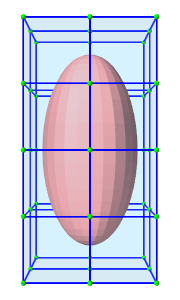 |
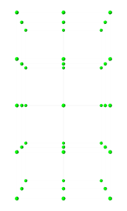 |
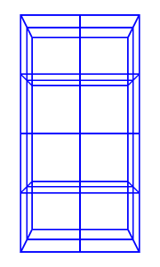 |
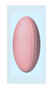 |
| (a) FEM model | (b) Nodes | (c) Elements | (d) Geometry |
6.1.2.1 Nodes
The set of nodes belonging to a finite element model can be obtained by the method
| PointList<FemNode3d> getNodes() |
Returns the list of FEM nodes. |
Nodes are implemented in the class FemNode3d, which is a subclass of Particle (Section 3.1). They are the main dynamic components of the finite element model. The key properties affecting simulation dynamics are:
| Property | Description |
|---|---|
| restPosition | The initial position of the node. |
| position | The current position of the node. |
| velocity | The current velocity of the node. |
| mass | The mass of the node. |
| dynamic | Whether the node is considered dynamic or parametric (e.g. boundary condition). |
Each of these properties has corresponding getXxx() and setXxx(...) functions to access and modify them.
The restPosition property defines the node’s position in the FEM model’s “natural” or “undeformed” state. Rest positions are used to compute an initial configuration for the model, from which strains are determined. A node’s rest position can be updated in code using the method: FemNode3d.setRestPosition(Point3d).
If any node’s rest positions are changed, the current values for stress and stiffness will become invalid. They can be manually updated using the method FemModel3d.updateStressAndStiffness() for the parent model. Otherwise, stress and stiffness will be automatically updated at the beginning of the next time step.
The properties position and velocity give the node’s current 3D state. These are common to all point-like particles, as is the mass property. Here, however, mass represents the lumped mass of the immediately surrounding material. Its value is initialized by equally dividing mass contributions from each adjacent element, given their densities. For a finer control of spatially-varying density, node masses can be set manually after FEM creation.
The FEM node’s dynamic property specifies whether or not the node is considered when computing the dynamics of the system. If not, it is treated as being parametrically controlled. This has implications when setting boundary conditions (Section 6.1.4).
6.1.2.2 Elements
Elements are the 3D volumetric spatial building blocks of the domain. Within each element, the displacement (or strain) field is interpolated from displacements at nodes:
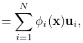 |
(6.2) |
where ![]() is the displacement of the
is the displacement of the ![]() th node that is adjacent to the
element, and
th node that is adjacent to the
element, and ![]() is referred to as the shape function (or
basis function) associated with that node. Elements are classified by
their shape, number of nodes, and shape function order (Table
6.1). ArtiSynth supports the following element types,
shown below with their node numberings:
is referred to as the shape function (or
basis function) associated with that node. Elements are classified by
their shape, number of nodes, and shape function order (Table
6.1). ArtiSynth supports the following element types,
shown below with their node numberings:
| TetElement | PyramidElement | WedgeElement | HexElement |
| QuadtetElement | QuadpyramidElement | QuadwedgeElement | QuadhexElement |
| Element Type | # Nodes | Order | # Integration Points |
|---|---|---|---|
| TetElement | 4 | linear | 1 |
| PyramidElement | 5 | linear | 5 |
| WedgeElement | 6 | linear | 6 |
| HexElement | 8 | linear | 8 |
| QuadtetElement | 10 | quadratic | 4 |
| QuadpyramidElement | 13 | quadratic | 5 |
| QuadwedgeElement | 15 | quadratic | 9 |
| QuadhexElement | 20 | quadratic | 14 |
The base class for all of these is FemElement3d. A numerical integration is performed within each element to create the (tangent) stiffness matrix. This integration is performed by evaluating the stress and stiffness at a set of integration points within each element, and applying numerical quadrature. The list of elements in a model can be obtained with the method
| RenderableComponentList<FemElement3d> getElements() |
Returns the list of volumetric elements. |
All objects of type FemElement3d have the following properties:
| Property | Description |
|---|---|
| density | Density of the element |
| material | An object that describes the constitutive law within the element (i.e. its stress-strain relationship). |
If left unspecified, the element’s density is inherited from the containing FemModel3d object. When set, the mass of the element is computed and divided amongst all its nodes, updating the lumped mass matrix.
6.1.2.3 Shell elements
Shell elements are additional 2D spatial building blocks which can be added to a model. They are typically used to model structures which are too thin to be easily represented by 3D volumetric elements, or to provide additional internal stiffness within a set of volumetric elements.
ArtiSynth presently supports the following shell element types, with the number of nodes, shape function order, and integration point count described in Table 6.2:
| Element Type | # Nodes | Order | # Integration Points |
|---|---|---|---|
| ShellTriElement | 3 | linear | 9 (3 if membrane) |
| ShellQuadElement | 4 | linear | 8 (4 if membrane) |
The base class for all shell elements is ShellElement3d, which contains the same density and material properties as FemElement3d, as well as the additional property defaultThickness, whose use will be described below.
The list of shell elements in a model can be obtained with the method
| RenderableComponentList<ShellElement3d> getShellElements() |
Returns the list of shell elements. |
Both the volumetric elements (FemElement3d) and the shell elements (ShellElement3d) derive from the base class FemElement3dBase. To obtain all the elements in an FEM model, both shell and volumetric, one may use the method
| ArrayList<FemElement3dBase> getAllElements() |
Returns a list of all elements. |
Each shell element can actually be instantiated in two forms:
-
•
As a regular shell element, which has a bending stiffness;
-
•
As a membrane element, which does not have bending stiffness.
Regular shell elements are implemented using the same extensible director formulation used by FEBio [12], and more specifically the front/back node formulation [13]. Each node associated with a (regular) shell element is assigned a director, which is a 3D vector providing a normal direction and virtual thickness at that node (Figure 6.3). This virtual thickness allows us to continue to use 3D materials to provide the constitutive laws that determine the shell’s stress/strain response, including its bending behavior. It also allows us to continue to use the element’s density to determine its mass.
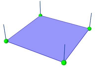
Director information is automatically assigned to a FemNode3d whenever one or more regular shell elements is connected to it. This information includes both the current value of the director, its rest value, and its velocity, with the difference between the first two determining the element’s bending strain. These quantities can be queried using the methods
For nodes which are not connected to regular shell elements, and therefore do not have director information assigned, these methods all return a zero-valued vector.
If not otherwise specified, the current and rest director values are
computed automatically from the surrounding (regular) shell elements,
with their value ![]() being computed from
being computed from
where ![]() is the value of the defaultThickness property and
is the value of the defaultThickness property and
![]() is the surface normal of the
is the surface normal of the ![]() -th surrounding regular shell
element.
However, if necessary, it is also possible to explicitly assign
these values, using the methods
-th surrounding regular shell
element.
However, if necessary, it is also possible to explicitly assign
these values, using the methods
ArtiSynth FEM nodes can currently support only one director, which is shared by all regular shell elements associated with that node. This effectively means that all such elements must belong to the same “surface”, and that two intersecting surfaces cannot share the same nodes.
As indicated above, shell elements can also be instantiated as membrane elements, which do not exhibit bending stiffness and therefore do not require director information. The regular/membrane distinction is specified in the element’s constructor. For example, ShellTriElement and ShellQuadElement each have constructors with the signatures:
The thickness argument specifies the defaultThickness property, while membrane determines whether or not the element is a membrane element.
While membrane elements do not require explicit director information stored at the nodes, they do make use of an inferred director that is parallel to the element’s surface normal, and has a constant length equal to the element’s defaultThickness property. This gives the element a virtual volume, which (as with regular elements) is used to determine 3D strains and to compute the element’s mass from its density.
6.1.2.4 Meshes
The geometry associated with a finite element model consists of a collection of meshes (e.g. PolygonalMesh, PolylineMesh, PointMesh) that move along with the model in a way that maintains the shape function interpolation equation (6.2) at each vertex location. These geometries can be used for visualizations, or for physical interactions like collisions. However, they have no physical properties themselves. FEM geometries will be discussed in more detail in Section 6.3. The list of meshes can be obtained with the method
6.1.3 Materials
The stress-strain relationship within each element is defined by a “material” delegate object, implemented by a subclass of FemMaterial. This material object is responsible for implementing the functions
which computes the stress tensor and (optionally) the tangent stiffness matrix at each integration point, based on the current local deformation at that point.
All supported materials are presented in detail in Section
6.10. The default material type is
LinearMaterial, which
linearly maps Cauchy strain ![]() onto Cauchy stress
onto Cauchy stress ![]() via
via
where ![]() is the elasticity tensor determined
from Young’s modulus and Poisson’s ratio. Anisotropic
linear materials are provided by
TransverseLinearMaterial
and
AnisotropicLinearMaterial.
Linear materials in ArtiSynth implement corotation, which removes the
rotation from the deformation gradient and allows Cauchy strain to be
applied to large
deformations [18, 16]. Nonlinear
hyperelastic materials are also supported, including
MooneyRivlinMaterial,
OgdenMaterial,
YeohMaterial,
ArrudaBoyceMaterial,
and
VerondaWestmannMaterial.
is the elasticity tensor determined
from Young’s modulus and Poisson’s ratio. Anisotropic
linear materials are provided by
TransverseLinearMaterial
and
AnisotropicLinearMaterial.
Linear materials in ArtiSynth implement corotation, which removes the
rotation from the deformation gradient and allows Cauchy strain to be
applied to large
deformations [18, 16]. Nonlinear
hyperelastic materials are also supported, including
MooneyRivlinMaterial,
OgdenMaterial,
YeohMaterial,
ArrudaBoyceMaterial,
and
VerondaWestmannMaterial.
6.1.4 Boundary conditions
Boundary conditions can be implemented in one of several ways:
-
1.
Explicitly setting FEM node positions/velocities
-
2.
Attaching FEM nodes to other dynamic components
-
3.
Enabling collisions
To enforce an explicit (Dirichlet) boundary condition for a set of nodes, their dynamic property must be set to false. This notifies ArtiSynth that the state of these nodes (both position and velocity) will be controlled parametrically. By disabling dynamics, a fixed boundary condition is applied. For a moving boundary, positions and velocities of the boundary nodes must be explicitly set every timestep. This can be accomplished with either a Controller (see Section 5.3) or an InputProbe (see Section 5.4). Note that both the position and velocity of the nodes should be explicitly set for consistency.
Another type of supported boundary condition is to attach FEM nodes to other components, including particles, springs, rigid bodies, and locations within other FEM elements. Here, the node is still considered dynamic, but its motion is coupled to that of the attached component through a constraint mechanism. Attachments will be discussed further in Section 6.4.
Finally, the boundary of an FEM can be constrained by enabling collisions with other components. This will be covered in Chapter 8.
6.2 FEM model creation
Creating a finite element model in ArtiSynth typically follows the pattern:
The main code block for the FEM setup should do the following:
-
•
Build the node/element structure
-
•
Set physical properties
-
–
density
-
–
damping
-
–
material
-
–
-
•
Set boundary conditions
-
•
Set render properties
Building the FEM structure can be done with the use of factory methods for simple shapes, by loading external files, or by writing code to manually assemble the nodes and elements.
6.2.1 Factory methods
For simple shapes such as beams and ellipsoids, there are factory methods to automatically build the node and element structure. These methods are found in the FemFactory class. Some common methods are
The inputs specify the dimensions, resolution, and potentially the type of element to use. The following code creates a basic beam made up of hexahedral elements:
6.2.2 Loading external FEM meshes
For more complex geometries, volumetric meshes can be loaded from external files. A list of supported file types is provided in Table 6.3. To load a geometry, an appropriate file reader must be created. Readers capable of reading FEM models implement the interface FemReader, which has the method
Additionally, many FemReader classes have static methods to handle the loading of files for convenience.
| Format | File extensions | Reader | Writer |
|---|---|---|---|
| ANSYS | .node, .elem | AnsysReader | AnsysWriter |
| ANSYS | .cdb | AnsysCdbReader | AnsysCdbWriter |
| TetGen | .node, .ele | TetGenReader | TetGenWriter |
| Abaqus | .inp | AbaqusReader | AbaqusWriter |
| Gmsh | .msh | GmshReader | GmshWriter |
| VTK (ASCII) | .vtk | VtkAsciiReader | – |
The following code snippet demonstrates how to load a model using the AnsysReader.
The method PathFinder.getSourceRelativePath() is used to find a path within the ArtiSynth source tree that is relative to the current model’s source file (Section 2.6). Note the try-catch block. Most of these readers throw an IOException if the read fails, and this must either be caught or thrown by the calling method.
As a different example, the following example creates a GmshReader and uses it to read in a model:
In this case, we create an actual reader instance instead of using one of the static methods, and the IOException is assumed to be handled outside the code fragment. Because the fem argument to readFem() is null, the reader creates a FEM model and returns it. The application must then set other properties for the FEM, such as the material and rendering properties.
One reason to create an actual reader instance is that it may provide access to various options related to the read. For example, both GmshReader and AnsysCdbReader supply the following:
6.2.3 Generating from surfaces
There are two ways an FEM model can be generated from a surface: by using a FEM mesh generator, and by extruding a surface along its normal direction.
ArtiSynth has the ability to interface directly with the TetGen library (http://tetgen.org) to create a tetrahedral volumetric mesh given a closed and manifold surface. The main Java class for calling TetGen directly is TetgenTessellator. The tessellator has several advanced options, allowing for the computation of convex hulls, and for adding points to a volumetric mesh. For simply creating an FEM from a surface, there is a convenience routine within FemFactory that handles both mesh generation and constructing a FemModel3d:
If quality ![]() , then points will be added in an attempt to bound the
maximum radius-edge ratio (see the -q switch for TetGen). According
to the TetGen documentation, the algorithm usually succeeds for a
quality ratio of 1.2.
, then points will be added in an attempt to bound the
maximum radius-edge ratio (see the -q switch for TetGen). According
to the TetGen documentation, the algorithm usually succeeds for a
quality ratio of 1.2.
It’s also possible to create thin layer of elements by extruding a surface along its normal direction.
For example, to create a two-layer slice of elements centered about a surface of a tendon mesh, one might use
For this type of extrusion, triangular faces become wedge elements, and quadrilateral faces become hexahedral elements.
Note: for extrusions, no care is taken to ensure element quality; if the surface has a high curvature relative to the total extrusion thickness, then some elements will be inverted.
6.2.4 Building elements in code
A finite element model’s structure can also be manually constructed in code. FemModel3d has the methods:
For an element to successfully be added, all its nodes must already have been added to the model. Nodes can be constructed from a 3D location, and elements from an array of nodes. A convenience routine is available in FemElement3d that automatically creates the appropriate element type given the number of nodes (Table 6.1):
Be aware of node orderings when supplying nodes. For linear elements, ArtiSynth uses a clockwise convention with respect to the outward normal for the first face, followed by the opposite node(s). To determine the correct ordering for a particular element, check the coordinates returned by the function FemElement3dBase.getNodeCoords(). This returns the concatenated coordinate list for an “ideal” element of the given type.
6.2.5 Example: a simple beam model
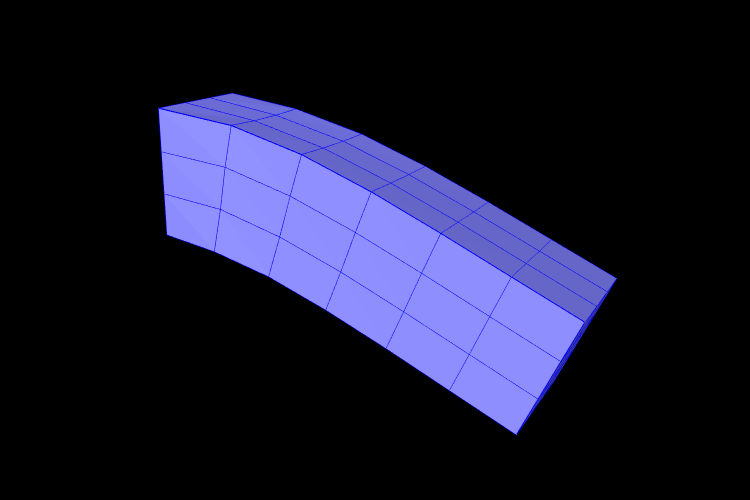
A complete application model that implements a simple FEM beam is given below.
This example can be found in artisynth.demos.tutorial.FemBeam. The build() method first creates a MechModel and FemModel3d. A FEM beam is created using a factory method on line 36. This beam is centered at the origin, so its length extends from -length/2 to length/2. The density, damping and material properties are then assigned.
On lines 45–49, a fixed boundary condition is set to the left-hand side of the beam by setting the corresponding nodes to be non-dynamic. Due to numerical precision, a small EPSILON buffer is required to ensure all left-hand boundary nodes are identified (line 46).
Rendering properties are then assigned to the FEM model on line 52. These will be discussed further in Section 6.12.
6.3 FEM Geometry
Associated with each FEM model is a list of geometry with the heading meshes. This geometry can be used for either display purposes, or for interactions such as collisions (Section 8.3.2). A geometry itself has no physical properties; its motion is entirely governed by the FEM model that contains it.
All FEM geometries are of type FemMeshComp, which stores a reference to a mesh object (Section 2.5), as well as attachment information that links vertices of the mesh to points within the FEM. The attachments enforce the shape function interpolation in Equation (6.2) to hold at each mesh vertex, with constant shape function coefficients.
6.3.1 Surface meshes
By default, every FemModel3d has an auto-generated geometry representing the “surface mesh”. The surface mesh consists of all un-shared element faces (i.e. the faces of individual elements that are exposed to the world), and its vertices correspond to the nodes that make up those faces. As the FEM nodes move, so do the mesh vertices due to the attachment framework.
The surface mesh can be obtained using one of the following functions in FemModel3d:
The first returns the surface complete with attachment information. The latter method directly returns the PolygonalMesh that is controlled by the FEM.
It is possible to manually set the surface mesh:
However, doing so is normally not necessary. It is always possible to add additional mesh geometries to a finite element model, and the visibility settings can be changed so that the default surface mesh is not rendered.
6.3.2 Embedding geometry within an FEM
Any geometry of type MeshBase can be added to a FemModel3d. To do so, first position the mesh so that its vertices are in the desired locations inside the FEM, then call one of the FemModel3d methods:
The latter is a convenience routine that also gives the newly embedded FemMeshComp a name.
6.3.3 Example: a beam with an embedded sphere
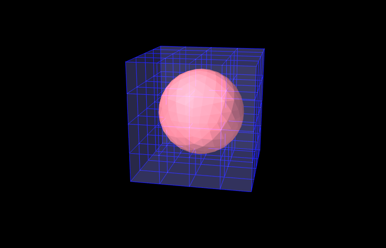
A complete model demonstrating embedding a mesh is given below.
This example can be found in artisynth.demos.tutorial.FemEmbeddedSphere. The model is very similar to FemBeam. A MechModel and FemModel3d are created and added. At line 41, a PolygonalMesh of a sphere is created using a factory method. The sphere is already centered inside the beam, so it does not need to be repositioned. At Line 42, the sphere is embedded inside model fem, creating a FemMeshComp with the name “sphere”. The full model is shown in Figure 6.5.
6.4 Connecting FEM models to other components
To couple FEM models to other dynamic components, the “attachment” mechanism described in Section 1.2.3 is used. This involves creating and adding to the model attachment components, which are instances of DynamicAttachment, as described in Section 3.9. Common point-based attachment classes are listed in Table 6.4.
| Attachment | Description |
|---|---|
| PointParticleAttachment | Attaches one “point” to one “particle” |
| PointFrameAttachment | Attaches one “point” to one “frame” |
| PointFem3dAttachment | Attaches one “point” to a linear combination of FEM nodes |
FEM models are connected to other model components by attaching their nodes to various components. This can be done by creating an attachment object of the appropriate type, and then adding it to the MechModel using
There are also convenience routines inside MechModel that will create the appropriate attachments automatically (see Section 3.9.1).
All attachments described in this section are based around FEM nodes. However, it is also possible to attach frame-based components (such as rigid bodies) directly to an FEM, as described in Section 6.6.
6.4.1 Connecting nodes to rigid bodies or particles
Since FemNode3d is a subclass of Particle, the same methods described in Section 3.9.1 for attaching particles to other particles and frames are available. For example, we can attach an FEM node to a rigid body using either a statement of the form
or the following equivalent statement which does the same thing:
Both of these create a PointFrameAttachment between a rigid body (called body) and an FEM node (called node) and then adds it to the MechModel mech.
6.4.2 Example: connecting a beam to a block
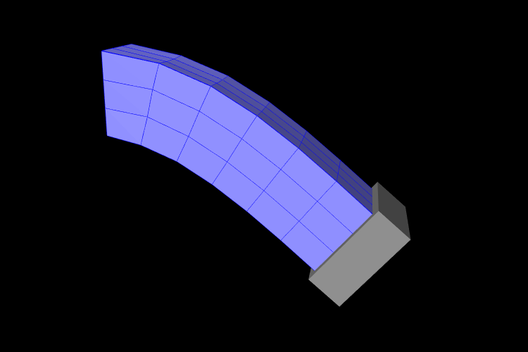
The following model demonstrates attaching an FEM beam to a rigid block.
This model extends the FemBeam example of Section 6.2.5. The build() method then creates and adds a RigidBody block (lines 18–20). On line 21, the block is repositioned to the side of the beam to prepare for the attachment. On lines 24–28, all right-most nodes of the beam are then set to be attached to the block using a PointFrameAttachment. In this case, the attachments are explicitly created. They could also have been attached using
6.4.3 Connecting nodes directly to elements
Typically, nodes do not align in a way that makes it
possible to connect them to other FEM models and/or points based on
simple point-to-node attachments. Instead, we use a different
mechanism that allows us to attach a point to an arbitrary location
within an FEM model. This is done using an attachment component of
type
PointFem3dAttachment, which
implements an attachment where the position ![]() and velocity
and velocity ![]() of the
attached point is determined by a weighted sum of the positions
of the
attached point is determined by a weighted sum of the positions ![]() and velocities
and velocities ![]() of selected fem nodes:
of selected fem nodes:
| (6.3) |
Any force ![]() acting on the attached point is then propagated back
to the nodes, according to the relation
acting on the attached point is then propagated back
to the nodes, according to the relation
| (6.4) |
where ![]() is the force acting on node
is the force acting on node ![]() due to
due to ![]() . This
relation can be derived based on the conservation of energy.
If
. This
relation can be derived based on the conservation of energy.
If ![]() is embedded within a single element, then the
is embedded within a single element, then the ![]() are
simply the element nodes and the
are
simply the element nodes and the ![]() are corresponding shape
function values; this is known as an element-based attachment.
On the other hand, as described below, it is sometimes desirable to
form an attachment using a more general set of nodes that extends
beyond a single element; this is known as a nodal-based
attachment (Section 6.4.8).
are corresponding shape
function values; this is known as an element-based attachment.
On the other hand, as described below, it is sometimes desirable to
form an attachment using a more general set of nodes that extends
beyond a single element; this is known as a nodal-based
attachment (Section 6.4.8).
An element-based attachment can be created using a code fragment of the form
First, a PointFem3dAttachment is created for the point pnt. Next, setFromElement() is used to determine the nodal weights within the element elem for the specified position (which in this case is simply the point’s current position). To do this, it computes the “natural coordinates” of the position within the element. For this to be guaranteed to work, the position should be on or inside the element. If natural coordinates cannot be found, the method will return false and the nearest estimated coordinates will be used instead. However, it is sometimes possible to find natural coordinates outside a given element as long as the shape functions are well-defined. Finally, the attachment is added to the model.
More conveniently, the exact same functionality is provided by the attachPoint() method in MechModel:
This creates an attachment identical to that created by the previous code fragment.
Often, one does not want to have to determine the element to which a point should be attached. In that case, one can call
or, equivalently,
This will find the nearest element to the node in question and use that to create the attachment. If the node is outside the FEM model, then it will be attached to the nearest point on the FEM’s surface.
6.4.4 Example: connecting two FEMs together
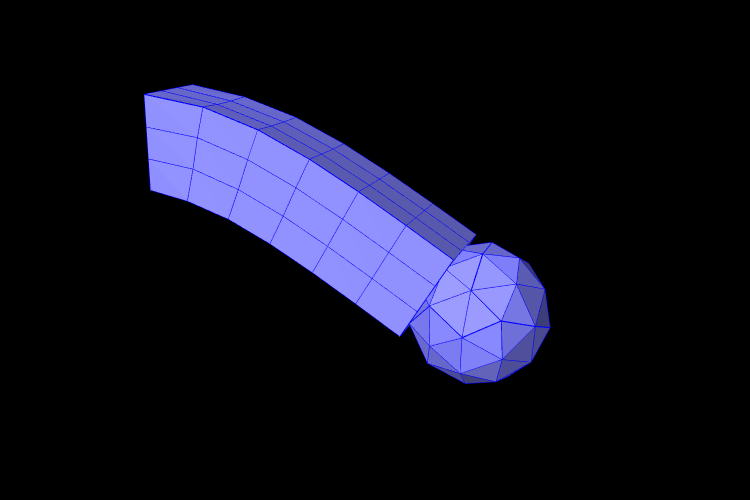
The following model demonstrates how to attach two FEM models together:
This example can be found in artisynth.demos.tutorial.FemBeamWithFemSphere. The model extends FemBeam, adding a finite element sphere and coupling them together. The sphere is created and added on lines 18–28. It is read from TetGen-generated files using the TetGenReader class. The model is then scaled to match the dimensions of the current model, and transformed to the right side of the beam. To create attachments, the code first checks for any nodes that belong to the sphere that fall inside the beam using the FemModel3d.findContainingElement(Point3d) method (line 36), which returns the containing element if the point is inside the model, or null if the point is outside. Internally, this spatial search uses a bounding volume hierarchy for efficiency (see BVTree and BVFeatureQuery). If the point is contained within the beam, then mech.attachPoint() is used to attach it to the nodes of the element (line 39).
6.4.5 Finding which nodes to attach
While it is straightforward to connect nodes to rigid bodies or other FEM nodes or elements, it is often necessary to determine which nodes to attach. This was evident in the example of Section 6.4.4, which attached nodes of an FEM sphere that were found to be inside an FEM beam.
As in that example, finding the nodes to attach can often be done using geometric queries. For example, we often select nodes based on how close they are to the other body we wish to attach to.
Various proximity queries are available for this task. To find the distance of a point to a polygonal mesh, we can use the following PolygonalMesh methods,
| double distanceToPoint(Point3d pnt) |
Returns the distance of pnt to the mesh. |
| int pointIsInside (Point3d pnt) |
Returns true if pnt is inside the mesh. |
where the latter method returns 1 if the point is inside and 0 otherwise. For checking the distance of an FEM node, pnt can be obtained from node.getPosition() (or possibly node.getRestPosition()). For example, to find all nodes within a distance tol of the surface of a rigid body, we could use the code fragment:
If we want to check only nodes that lie on the FEM surface, then we can filter them using the FemModel3d method isSurfaceNode():
Most of the mesh-based query methods work only for triangular meshes. The PolygonalMesh method isTriangular() can be used to determine if the mesh is triangular. If it is not, it can made triangular by calling triangulate(), although in general this should be done during model construction before the mesh-based component has been added to the model.
For connecting an FEM model to another FEM model, FemModel3d provides a number of query methods:
| Nearest element queries: | |
|---|---|
| FemElement3dBase findNearestElement( Point3d near, Point3d pnt) |
Find nearest element (shell or volumetric) to pnt. |
| FemElement3dBase findNearestElement( Point3d near, Point3d pnt, ElementFilter filter) |
Find nearest filtered element (shell or volumetric) to pnt. |
| FemElement3dBase findNearestSurfaceElement( Point3d near, Point3d pnt) |
Find nearest surface element (shell or volumetric) to pnt. |
| FemElement3d findNearestVolumetricElement ( Point3d near, Point3d pnt) |
Find nearest volumetric element to pnt. |
| ShellElement3d findNearestShellElement ( Point3d near, Point3d pnt) |
Find nearest shell element to pnt. |
| FemElement3d findContainingElement(Point3d pnt) |
Find volumetric element (if any) containing pnt. |
| Nearest node queries: | |
|---|---|
| FemNode3d findNearestNode ( Point3d pnt, double maxDist) |
Find nearest node to pnt that is within maxDist. |
| ArrayList<FemNode3d> findNearestNodes ( Point3d pnt, double maxDist) |
Find all nodes that are within maxDist of pnt. |
All the above queries are based on the FEM model’s current nodal
positions. The method
findNearestElement(near,pnt,filter) allows the application to
specify
a FemModel.ElementFilter to
restrict the elements that are searched.
The argument near that appears in some of the queries is an optional argument which, if not null, returns the location of the corresponding nearest point on the element. The distance from pnt to the element can then be found using
near.distance (pnt);
If the resulting distance is 0, then the point is on or inside the element. Otherwise, the point is outside the element, and if no element filters were used in the query, outside the FEM model itself.
Typically, it is preferred to attach a point to an element only if it lies on or inside an element. However, it is possible to attach points outside an element as long as the system is able to determine appropriate element “coordinates” for that point (which it may not be able to do if the point is far away). In addition, the motion behavior of an exterior attached point may sometimes appear counterintuitive.
The FemModel3d element and node queries can be used in a variety of ways.
findNearestNodes() can be used to find all nodes within a certain distance of a point, as part of the process of making nodal-based attachments (Section 6.4.8).
findNearestNode() is used in the FemMuscleBeam example (Section 6.9.5) to determine if a desired muscle point is near enough to a node to use that node directly, or if a marker should be created.
As another example, suppose we wish to connect the surface nodes of an FEM model femA to the surface elements of another model femB if they lie within a prescribed distance tol of the surface of femB. Then we could use the following code:
Finally, it is possible to identify nodes on the surface of an FEM model according to whether they belong to specific features, such as a smooth patch or a sharp edge line. Methods for doing this are provided as static methods in the class FemQuery, and include:
| Feature based node queries: | |
|---|---|
| ArrayList<FemNode3d> findPatchNodes ( FemModel3d fem, FemNode3d node0, double maxBendAng) |
Find nodes in patch defined by a maximum bend angle. |
| ArrayList<FemNode3d> findPatchBoundaryNodes ( FemModel3d fem, FemNode3d node0, double maxBendAng) |
Find the border nodes of a patch. |
| ArrayList<FemNode3d> findEdgeLineNodes ( FemModel3d fem, FemNode3d node0, double minBendAng, double maxEdgeAng, double allowBranching) |
Find the nodes along an edge defined by a minimum bend angle. |
Details of how these methods work are given in their API documentation. They use the notion of a bend angle, which is the absolute value of the angle between two faces about their common edge. A patch is defined by a collection of faces whose bend angles do not exceed a minimum value, while an edge line is a collection of edges with bend angles not below a maximum value. The feature methods start with an initial node (node0) and then grow the requested feature out from there. For example, suppose we have a regular hexahedral FEM grid, and we wish to find all the nodes on one of the faces. If we know one of the nodes on the face, then we can find all of the nodes using findPatchNodes:
Note that the feature query above uses a maximum bend angle of
![]() . Because grid faces are flat, this choice is somewhat
arbitrary; any angle larger than 0 (within machine precision) would also
work.
. Because grid faces are flat, this choice is somewhat
arbitrary; any angle larger than 0 (within machine precision) would also
work.
6.4.6 Selecting nodes in the viewer
Often, it is most convenient to select nodes in the ArtiSynth viewer. For this, a node selection tool is available (Figure 6.8), as described in the section “Selecting FEM nodes” of the ArtiSynth User Interface Guide). It allows nodes to be selected in various ways, including the usual click, drag box and elliptical selection tools, as well as specialized operations that select nodes based on patches, edge lines, and distances to other bodies. Once nodes have been selected, their numbers can be saved to a node number file which can then be read by a model’s build() method to determine which nodes to connect to some body.
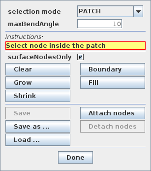
Node number files are text files with a very simple format, consisting of integers (the node numbers), separated by white space. There is no limit to how many numbers can appear on a line but typically this is limited to ten or so to make the file more readable. Optionally, the numbers can be surrounded by square brackets ([ ]). The special character ‘#’ is a comment character, commenting out all characters from itself to the end of the current line. For a file containing the node numbers 2, 12, 4, 8, 23 and 47, the following formats are all valid:
Once node numbers have been identified in the viewer and saved in a file, they can be read by the build() method using a NodeNumberReader. For convenience, this class supplies two static methods for extracting the FEM nodes specified by the numbers in a file:
| static ArrayList<FemNode3d> read( File file, FemModel3d fem) |
Returns nodes in fem corresponding to file’s numbers. |
| static ArrayList<FemNode3d> read( String filePath, FemModel3d fem) |
Returns nodes in fem corresponding to file’s numbers. |
Extracted nodes can be used to set boundary conditions or form connections with other bodies. For example, suppose we wish to connect a face of an FEM model fem to a rigid body block, using a set of nodes specified in a file called faceNodes.txt. A code fragment to accomplish this could be the following:
The process of selecting nodes in the viewer, saving them in a file, and using them in a model can be done iteratively: if the selected nodes need to be adjusted, one can reopen the node selection tool, load the selection from file, adjust the selection, and resave the file, without needing to make any modifications to the model’s build() code.
If desired, one can also determine a set of nodes in code, and then write their numbers to a file using the class NodeNumberWriter, which supplies static methods for writing number files:
| static void write( String filePath, Collection<FemNode3d> nodes) |
Writes the numbers of nodes to the specified file. |
| static void write( File file, Collection<FemNode3d> nodes) |
Writes the numbers of nodes to file. |
| static void write( File file, Collection<FemNode3d> nodes, int maxCols, int flags) |
Writes the numbers of nodes to file, using the specified number of columns and format flags. |
For example:
6.4.7 Example: two bodies connected by an FEM “spring”
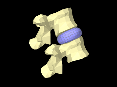
The LumbarFrameSpring example in Section 3.7.4 uses a frame spring to connect two simplified lumbar vertebrae. However, it is also possible to use an FEM model in place of a frame spring, possibly providing a more realistic model of the intervertebral disc. A simple model which does this is defined in
artisynth.demos.tutorial.LumbarFEMDisk
The initial source code is similar to that for LumbarFrameSpring, but differs in the section where the FEM disk replaces the FrameSpring:
The simplified FEM model representing the “disk” is created at lines 57-61, using a torus-shaped model created by FemFactory. It is then repositioned using transformGeometry() ( Section 4.7) to place it between the vertebrae (line 64-66). After the FEM model is positioned, we find which nodes are within a distance tol of each vertebral surface and attach them to the appropriate body (lines 69-81).
To run this example in ArtiSynth, select All demos > tutorial > LumbarFEMDisk from the Models menu. The model should load and initially appear as in Figure 6.9. The behavior is best seen by running the model and using the pull controller to exert forces on the upper vertebra.
6.4.8 Nodal-based attachments
The example of Section 6.4.4 uses element-based attachments to connect the nodes of one FEM to elements of another. As mentioned above, element-based attachments assume that the attached point is associated with a specific FEM model element. While this often gives good results, there are situations where it may be desirable to distribute the connection more broadly among a larger set of nodes.
In particular, this is sometimes the case when connecting FEM models to point-to-point springs. The end-point of such a spring may end up exerting a large force on the FEM, and then if the number of nodes to which the end-point is attached are too small, the resulting forces on these nodes (Equation 6.4) may end up being too large. In other words, it may be desirable to distribute the spring’s force more evenly throughout the FEM model.
To handle such situations, it is possible to create a nodal-based attachment in which the nodes and weights are explicitly specified. This involves explicitly creating a PointFem3dAttachment for the point or particle to be attached and the specifying the nodes and weights directly,
where nodes and weights are arrays of FemNode and double, respectively. It is up to the application to determine these.
PointFem3dAttachment provides several methods for explicitly specifying nodes and weights. The signatures for these include:
The last two methods determine the weights automatically, using an
inverse-distance-based calculation in which each weight ![]() is initially computed as
is initially computed as
| (6.4) |
where ![]() is the distance from node
is the distance from node ![]() to pos and
to pos and
![]() is the maximum distance. The weights are then
adjusted to ensure that they sum to one and that the weighted sum of
the nodes equals pos. In some cases, the specified nodes
may not provide enough support for the last condition to be
met, in which case the methods return false.
is the maximum distance. The weights are then
adjusted to ensure that they sum to one and that the weighted sum of
the nodes equals pos. In some cases, the specified nodes
may not provide enough support for the last condition to be
met, in which case the methods return false.
6.4.9 Example: element vs. nodal-based attachments
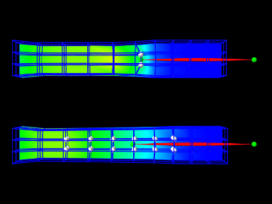
The model demonstrating the difference between element and nodal-based attachments is defined in
artisynth.demos.tutorial.PointFemAttachment
It creates two FEM models, each with a single point-to-point spring attached to a particle at their center. The model at the top (fem1 in the code below) is connected to the particle using an element-based attachment, while the lower model (fem2 in the code) is connected using a nodal-based attachment with a larger number of nodes. Figure 6.10 shows the result after the model is run until stable. The element-based attachment results in significantly higher deformation in the immediate vicinity around the attachment, while for the nodal-based attachment, the deformation is distributed much more evenly through the model.
The build method and some of the auxiliary code for this model is shown below. Code for the other auxiliary methods, including addFem(), addParticle(), addSpring(), and setAttachedNodesWhite(), can be found in the actual source file.
The build() method begins by creating a MechModel and then adding to it two FEM beams (created using the auxiliary method addFem()). Rendering of each FEM model’s surface is then set up to show strain values (setSurfaceRendering(), lines 41 and 43). The surface meshes themselves are also redefined to exclude the frontmost elements, allowing the strain values to be displayed closer to the model centers. This redefinition is done using calls to createSurfaceMesh() (lines 40, 41) with a custom ElementFilter defined at lines 3-12.
Next, the end-point particles for the axial springs are created (using the auxiliary method addParticle(), lines 46-49), and particle m1 is attached to fem1 using mech.attachPoint() (line 52), which creates an element-based attachment at the point’s current location. Point m2 is then attached to fem2 using a nodal-based attachment. The nodes for these are collected as the union of all nodes for a specified set of elements (lines 58-59, and the method collectNodes() defined at lines 16-25). These are then used to create a nodal-based attachment (lines 61-63), where the weights are determined automatically using the method associated with equation (6.4).
Finally, the springs are created (auxiliary method addSpring(), lines 66-67), the nodes associated for each attachment are set to render as white spheres (setAttachedNodesWhite(), lines 70-71), and the particles are set to render as green spheres.
To run this example in ArtiSynth, select All demos > tutorial > PointFemAttachment from the Models menu. Running the model will cause it to settle into the state shown in Figure 6.10. Selecting and dragging one of the spring anchor points at the right will cause the spring tension to vary and further illustrate the difference between the element and nodal-based attachments.
6.5 FEM markers
Just as there are FrameMarkers to act as anchor points on a frame or rigid body (Section 3.2.1), there are also FemMarkers that can mark a point inside a finite element. They are frequently used to provide anchor points for attaching springs and forces to a point inside an element, but can also be used for graphical purposes.
FEM markers are implemented by the class FemMarker, which is a subclass of Point. They are essentially massless points that contain their own attachment component, so when creating and adding a marker there is no need to create a separate attachment component.
Within the component hierarchy, FEM markers are typically stored in the markers container of their associated FEM model. They can be created and added using a code fragment of the form
This creates a marker at the location ![]() (in world
coordinates), calls setFromFem() to attach it to the nearest
element in the FEM model ( which is either the containing element or
the nearest element on the model’s surface), and then adds it to the
markers list.
(in world
coordinates), calls setFromFem() to attach it to the nearest
element in the FEM model ( which is either the containing element or
the nearest element on the model’s surface), and then adds it to the
markers list.
If the marker’s attachment has not already been set when addMarker() is called, then addMarker() will call setFromFem() automatically. Therefore the above code fragment is equivalent to the following:
Alternatively, one may want to explicitly specify the nodes associated with the attachment, as described in Section 6.4.8:
There are a variety of methods available to set the attachment, mirroring those available in the implementing class PointFem3dAttachment:
The last two methods compute nodal weights automatically, as described in Section 6.4.8, based on the marker’s currently assigned position. If the supplied nodes do not provide sufficient support, then the methods return false.
Another set of convenience methods are supplied by FemModel3d, which combine these with the addMarker() call:
For example, one can do
FemModel3d also provides the following additional methods to add markers and manage its marker container:
| void addMarker (Point3d pos) |
Adds a marker at pos (in world coords). |
| void addMarker (Point3d pos, boolean project) |
Adds a marker; projects to FEM if outside and project is true. |
| boolean removeMarker (FemMarker mkr) |
Remove the marker mkr; return true if it was present. |
| void clearMarkers () |
Remove all markers. |
| PointList<FemMarker> markers() |
Return the markers container. |
FemMarker is a subclass of Point, and so has the same accessors for querying position and velocity and setting forces as described in Section 3.1.1.
6.5.1 Example: attaching an FEM beam to a muscle
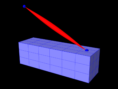
A complete application model that employs a fem marker as an anchor for a spring is given below.
This example can be found in artisynth.demos.tutorial.FemBeamWithMuscle. This model extends the FemBeam example, adding a FemMarker for the spring to attach to. The method createMarker(...) on lines 29–35 is used to create and add a marker to the FEM. Since the element is initially set to null, when it is added to the FEM, the model searches for the containing or nearest element. The loaded model is shown in Figure 6.11.
6.6 Frame attachments
It is also possible to attach frame components, including rigid bodies, directly to FEM models, using the attachment component FrameFem3dAttachment. Analogously to PointFem3dAttachment, the attachment is implemented by connecting the frame to a set of FEM nodes, and attachments can be either element-based or nodal-based. The frame’s origin is computed in the same way as for point attachments, using a weighted sum of node positions (Equation 6.3), while the orientation is computed using a polar decomposition on a deformation gradient determined from either element shape functions (for element-based attachments) or a Procrustes type analysis using nodal rest positions (for nodal-based attachments).
An element-based attachment can be created using either a code fragment of the form
or, equivalently, the attachFrame() method in MechModel:
This attaches the frame frame to the nodes of the FEM element elem. As with PointFem3dAttachment, if the frame’s origin is not inside the element, it may not be possible to accurately compute the internal nodal weights, in which case setFromElement() will return false.
In order to have the appropriate element located automatically, one can instead use
or, equivalently,
As with point-to-FEM attachments, it may be desirable to create a nodal-based attachment in which the nodes and weights are not tied to a specific element. The reasons for this are generally the same as with nodal-based point attachments (Section 6.4.8): the need to distribute the forces and moments acting on the frame across a broader set of element nodes. Also, element-based frame attachments use element shape functions to determine the frame’s orientation, which may produce slightly asymmetric results if the frame’s origin is located particularly close to a specific node.
FrameFem3dAttachment provides several methods for explicitly specifying nodes and weights. The signatures for these include:
Unlike their counterparts in PointFem3dAttachment, the first two methods also require the current desired pose of the frame TFW (in world coordinates). This is because while nodes and weights will unambiguously specify the frame’s origin, they do not specify the desired orientation.
6.6.1 Example: attaching frames to an FEM beam
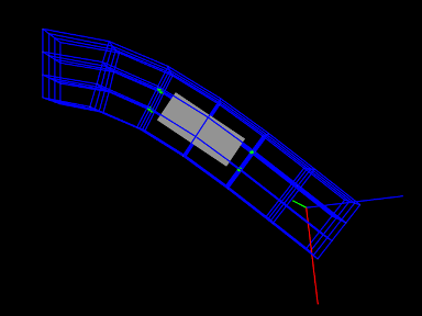
A model illustrating how to connect frames to an FEM model is defined in
artisynth.demos.tutorial.FrameFemAttachment
It creates an FEM beam, along with a rigid body block and a massless coordinate frame, that are then attached to the beam using nodal and element-based attachments. The build method is shown below:
Lines 3-22 create a MechModel and populate it with an FEM beam and a rigid body box. Next, a basic Frame is created, with a specified pose and an axis length of 0.3 (to allow it to be seen), and added to the MechModel (lines 25-28). It is then attached to the FEM beam using an element-based attachment (line 30). Meanwhile, the box is attached to using a nodal-based attachment, created from all the nodes associated with elements 22 and 31 (lines 33-36). Finally, all attachment nodes are set to be rendered as green spheres (lines 39-41).
To run this example in ArtiSynth, select All demos > tutorial > FrameFemAttachment from the Models menu. Running the model will cause it to settle into the state shown in Figure 6.12. Forces can interactively be applied to the attached block and frame using the pull tool, causing the FEM model to deform (see the section “Pull Manipulation” in the ArtiSynth User Interface Guide).
6.6.2 Attached frames
A FemAttachedFrame is an AttachedFrame that is connected to a FemModel3d, analogous to FrameAttachedFrame components that are connected to Frames (Section 3.10.1). The attachment is element-based: the frame’s position and orientation track a weighted combination of the surrounding FEM nodes, using natural coordinates within the enclosing (or nearest) element. The frame therefore moves and changes orientation as the FE model deforms.
FemAttachedFrame objects can be created using the constructors
| FemAttachedFrame () | |
| FemAttachedFrame (RigidTransform3d TFW) | |
| FemAttachedFrame (FemElement3dBase elem, RigidTransform3d TFW) |
where FemAttachedFrame() creates a default frame with no attachment, FemAttachedFrame(TFW) sets the initial world pose to TFW, and FemAttachedFrame(elem,TFW) also attaches the frame to the specified element. Once created, the nature of the FE attachment can be set or changed using
| void setFromFem (FemModel3d fem) |
Attaches to the nearest element in fem. |
| void setFromElement (FemElement3dBase elem) |
Attaches to elem using natural coordinates computed from the frame’s current pose. |
| boolean setFromNodes ( Collection<FemNode3d> nodes, VectorNd weights) |
Attaches to the specified nodes using the given weights. |
| boolean setFromNodes ( FemNode3d[] nodes, double[] weights) |
Attaches to the specified nodes using the given weights. |
| boolean setFromNodes (Collection<FemNode3d> nodes) |
Attaches to the specified nodes using inverse-distance weighting based on the frame’s current pose. |
| boolean setFromNodes (FemNode3d[] nodes) |
Attaches to the specified nodes using inverse-distance weighting based on the frame’s current pose. |
The setFromNodes() methods mirror those available for FemMarker (Section 6.4.8): the first two take explicit weights, while the last two determine weights automatically using inverse-distance weighting as described by equation (6.4).
Once created, the attached frame must be added to the MechModel hierarchy. One choice is to add them directly to the FE model to which they are attached. Each FemModel3d maintains an attachedFrames container, which may be managed using the following FemModel3d methods:
| void addAttachedFrame (FemAttachedFrame frm) |
Adds an existing frame, attaching it to the nearest element if not already attached to this model. |
| void addAttachedFrame ( FemAttachedFrame frm, FemElement3dBase elem) |
Adds an existing frame, attaching it to the specified element. |
| FemAttachedFrame addAttachedFrame ( RigidTransform3d TFW) |
Creates a new FemAttachedFrame located at world pose |
| boolean removeAttachedFrame (FemAttachedFrame frm) |
Removes frm from the list; returns true if present. |
| void clearAttachedFrames () |
Removes all frames from the attachedFrames list. |
| RenderableComponentList<FemAttachedFrame> getAttachedFrames () |
Returns the attachedFrames sub-list. |
Alternatively, attached frames can be added to the MechModel’s frames container, which is managed using the MechModel methods
| void addFrame (Frame frame) |
Adds frame frame to the container. |
| boolean removeFrame (Frame frame) |
Removes frame frame from the container. |
| void clearFrames() |
Removes all frames. |
| RenderableComponentList<Frame> frames() |
Returns the frames container. |
6.6.3 Example: attached frames for an FE model
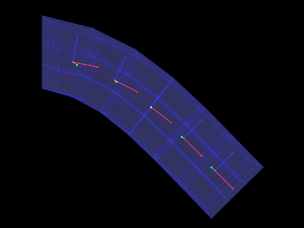
The following model demonstrates how to add FemAttachedFrames to an FEM beam:
This example can be found in artisynth.demos.tutorial.FemAttachedFrames.
It extends FemBeam (Section 6.2.5), adding five evenly-spaced
FemAttachedFrames along the beam’s local ![]() -axis (lines 20–27). Each
frame is positioned at a world-coordinate pose computed from the beam’s length,
and added to the FEM model using fem.addAttachedFrame(TFW), which
automatically finds and attaches to the nearest element. The frames are
rendered as solid arrow triads with an axis length of 0.12. Finally, the FEM
surface is made semi-transparent (line 29) so the embedded frames are visible.
-axis (lines 20–27). Each
frame is positioned at a world-coordinate pose computed from the beam’s length,
and added to the FEM model using fem.addAttachedFrame(TFW), which
automatically finds and attaches to the nearest element. The frames are
rendered as solid arrow triads with an axis length of 0.12. Finally, the FEM
surface is made semi-transparent (line 29) so the embedded frames are visible.
To run this example in ArtiSynth, select All demos > tutorial > FemAttachedFrames from the Models menu. The model should load and initially appear as in Figure 6.13. Running the model will cause the beam to fall under gravity, with all attached frames moving and rotating to track the deformation of the beam.
6.6.4 Adding joints to FEM models
The ability to connect frames to FEM models, as described in Section 6.6, makes it possible to interconnect different FEM models directly using joints, as described in Section 3.4. This is done internally by using FrameFem3dAttachments to connect frames C and D of the joint (Figure 3.9) to their respective FEM models.
As indicated in Section 3.4.3, most joints have a constructor of the form
that creates a joint connecting bodyA to bodyB, with the initial pose of the D frame given (in world coordinates) by TDW. The same body and transform settings can be made on an existing joint using the setBodies() methods also described in Section 3.4.3. For these constructors and methods, it is possible to specify FEM models for bodyA and/or bodyB. Internally, the joint then creates a FrameFem3dAttachment to connect frame C and/or D of the joint (See Figure 3.9) to the corresponding FEM model.
However, unlike joints involving rigid bodies or frames, there are no
associated ![]() or
or ![]() transforms (since there is no fixed
frame within an FEM to define such transforms). Methods or
constructors which utilize
transforms (since there is no fixed
frame within an FEM to define such transforms). Methods or
constructors which utilize ![]() or
or ![]() can therefore
not be used with FEM models.
can therefore
not be used with FEM models.
Sometimes, the default FrameFem3dAttachment attachment created by the joint constructor (or the setBodies() method) is not suitable, because the attachment’s support must be distributed across a node set that is either larger, or distributed differently. In that case, one may create a custom FrameFem3dAttachment using a specified set of nodes (and weights, if needed), as described in Section 6.6. This can then be used to connect the joint to the FEM via one of the setBodies() or setBodyA/B() methods that accepts custom FrameAttachments:
Note that when being used as a joint connector, FrameFem3dAttachment does not need to be associated with an actual frame component.
6.6.5 Example: two FEM beams connected by a joint
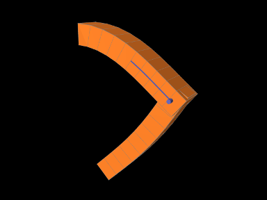
A model connecting two FEM beams by a joint is defined in
artisynth.demos.tutorial.JointedFemBeams
It creates two FEM beams and connects them via a special slotted-revolute joint. The build method is shown below:
Lines 3-16 create a MechModel and populate it with two FEM beams, fem1 and fem2, using an auxiliary method addFem() defined in the model source file. The leftmost nodes of fem1 are set fixed. A SlottedRevoluteJoint is then created to interconnect fem1 and fem2 at a location specified by TDW (lines 19-21). Lines 24-29 set some parameters for the joint, along with various render properties.
To run this example in ArtiSynth, select All demos > tutorial > JointedFemBeams from the Models menu. Running the model will cause it to drop and flex under gravity, as shown in Figure 6.14. Forces can interactively be applied to the beams using the pull tool (see the section “Pull Manipulation” in the ArtiSynth User Interface Guide).
6.7 Incompressibility
FEM incompressibility within ArtiSynth is enforced by trying to ensure that the volume of an FEM remains locally constant. This, in turn, is accomplished by constraining nodal velocities so that the local volume change, or divergence, is zero (or close to zero). There are generally two ways to do this:
-
•
Hard incompressibility, which sets up explicit constraints on the nodal velocities;
-
•
Soft incompressibility, which uses a restoring pressure based on a potential field to try to keep the volume constant.
Both of these methods operate independently, and both can be used either separately or together. Generally speaking, hard incompressibility will result in incompressibility being more rigorously enforced, but at the cost of increased computation time and (sometimes) less stability. Soft incompressibility allows the application to control the restoring force used to enforce incompressibility, usually by adjusting the value of the bulk modulus material property. As the bulk modulus is increased, soft incompressibility starts to act more like ‘hard’ incompressibility, with an infinite bulk modulus corresponding to perfect incompressibility. However, very large bulk modulus values will generally produce stability problems.
Incompressibility is not currently implemented for shell elements. Applying hard incompressibility to a shell element will have no effect on its behavior. If soft incompressibility is applied, by supplying the element with an incompressible material, then only the deviatoric component of that material will have any effect; the dilational component will generate no stress.
6.7.1 Volume regions and locking
Both hard and soft incompressibility can be applied to different regions of local volume. From larger to smaller, these regions are:
-
•
Nodal - the local volume surrounding each node;
-
•
Element - the volume of each element;
-
•
Full - the volume at each integration point.
Element-based incompressibility is the standard method generally seen
in the literature. However, it tends not to work well for
tetrahedral meshes, because constraining the volume of each tet in a
tetrahedral mesh tends to over constrain the system. This is because
the number of tets in a large tetrahedral mesh is often ![]() ,
where
,
where ![]() is the number of nodes, and so putting a volume constraint
on each element may result in
is the number of nodes, and so putting a volume constraint
on each element may result in ![]() constraints, which exceeds the
constraints, which exceeds the
![]() degrees of freedom (DOF) in the FEM. This overconstraining results in an
artificially increased stiffness known as locking. Because of
locking, for tetrahedrally based meshes it may be better to use
nodal-based incompressibility, which creates a single volume constraint
around each node, resulting in only
degrees of freedom (DOF) in the FEM. This overconstraining results in an
artificially increased stiffness known as locking. Because of
locking, for tetrahedrally based meshes it may be better to use
nodal-based incompressibility, which creates a single volume constraint
around each node, resulting in only ![]() constraints, leaving
constraints, leaving ![]() DOF
to handle the remaining deformation. However, nodal-based
incompressibility is computationally more costly than element-based
and may not be as stable.
DOF
to handle the remaining deformation. However, nodal-based
incompressibility is computationally more costly than element-based
and may not be as stable.
Generally, the best solution for incompressible problems is to use
element-based incompressibility with a mesh consisting of hexahedra,
or primarily hexahedra and a mix of other elements (the latter
commonly being known as a hex dominant mesh). For hex-based
meshes, the number of elements is roughly equal to the number of
nodes, and so adding a volume constraint for each element imposes ![]() constraints on the model, which (like nodal incompressibility)
leaves
constraints on the model, which (like nodal incompressibility)
leaves ![]() DOF to handle the remaining deformation.
DOF to handle the remaining deformation.
Full incompressibility tries to control the volume at each integration point within each element, which almost always results in a large number of volumetric constraints and hence locking. It is therefore not commonly used and is provided mostly for debugging and diagnostic purposes.
6.7.2 Hard incompressibility
Hard incompressibility is controlled by the incompressible property of the FEM, which can be set to one of the following values of the enumerated type FemModel.IncompMethod:
- OFF
-
No hard incompressibility enforced.
- ELEMENT
-
Element-based hard incompressibility enforced (Section 6.7.1).
- NODAL
-
Nodal-based hard incompressibility enforced (Section 6.7.1).
- AUTO
-
Selects either ELEMENT or NODAL, with the former selected if the number of elements is less than or equal to the number of nodes.
- ON
-
Same as AUTO.
Hard incompressibility uses explicit constraints on the nodal velocities to enforce the incompressibility, which increases computational cost. Also, if the number of constraints is too large, perturbed pivot errors may be encountered by the solver. However, hard incompressibility can in principle handle situations where complete incompressibility is required. It is equivalent to the mixed u-P formulation used in commercial FEM codes (such as ANSYS), and the Lagrange multipliers computed for the constraints are pressure impulses.
Hard incompressibility can be applied in addition to soft incompressibility, in which case it will provide additional incompressibility enforcement on top of that provided by the latter. It can also be applied to linear materials, which are not themselves able to emulate true incompressible behavior (Section 6.7.4).
6.7.3 Soft incompressibility
Soft incompressibility enforces incompressibility using a restoring
pressure that is controlled by a volume-based energy potential. It is
only available for FEM materials that are subclasses of
IncompressibleMaterial.
The energy potential ![]() is a function of the determinant
is a function of the determinant ![]() of the
deformation gradient, and is scaled by the material’s bulk modulus
of the
deformation gradient, and is scaled by the material’s bulk modulus
![]() . The restoring pressure
. The restoring pressure ![]() is given by
is given by
| (6.4) |
Different potentials can be selected by setting the bulkPotential property of the incompressible material, whose value is an instance of IncompressibleMaterial.BulkPotential. Currently there are two different potentials:
- QUADRATIC
-
The potential and associated pressure are given by
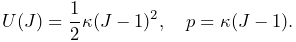
(6.5) - LOGARITHMIC
-
The potential and associated pressure are given by
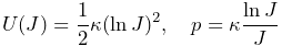
(6.6)
The default potential is QUADRATIC, which may provide slightly improved stability characteristics. However, we have not noticed significant differences between the two potentials in practice.
How soft incompressibility is applied within an FEM model is controlled by the FEM’s softIncompMethod property, which can be set to one of the following values of the enumerated type FemModel.IncompMethod:
- ELEMENT
-
Element-based soft incompressibility enforced (Section 6.7.1).
- NODAL
-
Nodal-based soft incompressibility enforced (Section 6.7.1).
- AUTO
-
Selects either ELEMENT or NODAL, with the former selected if the number of elements is less than or equal to the number of nodes.
- FULL
-
Incompressibility enforced at each integration point (Section 6.7.1).
6.7.4 Incompressibility and linear materials
Within a linear material, incompressibility is controlled by Poisson’s
ratio ![]() , which for isotropic materials can assume a value in the
range
, which for isotropic materials can assume a value in the
range ![]() . This specifies the amount of transverse contraction
(or expansion) exhibited by the material as it compressed or extended
along a particular direction. A value of
. This specifies the amount of transverse contraction
(or expansion) exhibited by the material as it compressed or extended
along a particular direction. A value of ![]() allows the material to be
compressed or extended without any transverse contraction or
expansion, while a value of
allows the material to be
compressed or extended without any transverse contraction or
expansion, while a value of ![]() in theory indicates a perfectly
incompressible material. However, setting
in theory indicates a perfectly
incompressible material. However, setting ![]() in practice
causes a division by zero, so only values close to 0.5 (such as 0.49)
can be used.
in practice
causes a division by zero, so only values close to 0.5 (such as 0.49)
can be used.
Moreover, the incompressibility only applies to small displacements,
so that even with ![]() it is still possible to squash a linear
FEM completely flat if enough force is applied. If true incompressible
behavior is desired with a linear material, then one must also use
hard incompressibility (Section 6.7.2).
it is still possible to squash a linear
FEM completely flat if enough force is applied. If true incompressible
behavior is desired with a linear material, then one must also use
hard incompressibility (Section 6.7.2).
6.7.5 Using incompressibility in practice
As mentioned above, when modeling incompressible models, we have found that the best practice is to use, if possible, either a hex or hex-dominant mesh, along with element-based incompressibility.
Hard incompressibility allows the handling of full incompressibility but at the expense of greater computational cost and often less stability. When modeling biomechanical materials, it is often permissible to use only soft incompressibility, partly since biomechanical materials are rarely completely incompressible. When implementing soft incompressibility, it is common practice to set the bulk modulus to something like 100 times the other (deviatoric) stiffnesses of the material.
We have found stability behavior to be complex, and while hard incompressibility often results in less stable behavior, this is not always the case: in some situations the stronger enforcement afforded by hard incompressibility actually improves stability.
6.8 Varying and augmenting material behaviors
The default material used by all elements of an FEM model is supplied by the model’s material property. However, it is often the case that one wishes to specify different material behaviors for different sets of elements within an FEM model. This may be particularly true when combining volumetric and shell elements.
There are several ways to vary material behavior within a model. These include:
-
•
Setting an explicit material for specific elements, using their material property. An element’s material is null by default, but if set to a material, it will override the default material supplied by the FEM model. While this method is quite straightforward, it does have one disadvantage: because material settings are copied by each element, subsequent interactive or online changes to the material require resetting the material in all the affected elements.
-
•
Binding one or more material parameters to a field. Sometimes certain material parameters, such as stiffness quantities or direction information, may need to vary across the FEM domain. While sometimes this can be handled by setting material properties for specific elements, it may be more convenient to bind the varying properties to a field, which can specify varying values over a domain composed of either a regular grid or an FEM mesh. Only one material needs to be used, and any properties which are not bound can be adjusted interactively or online. Fields and their bindings are described in detail in Chapter 7.
-
•
Adding augmenting material behaviors using MaterialBundles. A material bundle may be specified either for all elements, or for a subset of them, and each provides one material (via its own material property) whose behavior is added to that of the indicated elements. This also provides an easy way to combine the behaviors of two of more materials in the same element. One also has the option of setting the material property of the certain elements to NullMaterial, so that only the augmenting material(s) are applied.
-
•
Adding muscle behaviors using MuscleBundles. This is analogous to using MaterialBundles, except that MuscleBundles are restricted to using an instance of a MuscleMaterial, and include support for handling the excitation value, as well as the activation directions (which usually vary across the FEM domain). MuscleBundles are only present in the FemMuscleModels subclass of FemModel3d, and are described in detail in Section 6.9.
The remainder of this section will discuss MaterialBundles.
Adding a MaterialBundle to an FEM model is illustrated by the following code fragment:
Once added, the stress computed by the bundle’s material will be added to the stress computed by any other materials which are active for the bundle’s elements.
When deciding what elements to add to a bundle, one is free to choose any means necessary. The example above inspects all the volumetric elements in the FEM. To instead inspect all the shell elements, or all volumetric and shell elements, one could use the code fragments such as the following:
Of course, if the elements are known through other means, then they can be added directly.
The element composition of a bundle can be controlled by the methods
It is also possible to create a MaterialBundle whose material is added to all the FEM elements. This can done either by using one of the following constructors
with useAllElements set to true, or by calling the method
When a bundle is set to use all the FEM elements, it clears its own element list, and one is not permitted to add elements using addElement(elem).
After a bundle has been created, it is possible to get or set its material property using the methods
Again, because materials are copied internally, any modification to a material after it has been used as an input to setMaterial() will not be noticed by the bundle. Instead, one should modify the material before calling setMaterial(), or modify the copied material which can be obtained by calling getMaterial() or by storing the value returned by setMaterial().
Finally, a MaterialBundle is a renderable component. Setting its elementWidgetSize property to a value greater than zero will cause the rendering of all its elements, using a solid widget representation of each at a scale controlled by elementWidgetSize: 0.5 for half size, 1.0 for full size, etc. The color of the widgets is controlled by the faceColor property of the bundle’s renderProps. Being able to render the elements makes it easy to select the bundle and visualize which elements it contains.
6.8.1 Example: FEM sheet with a stiff spine
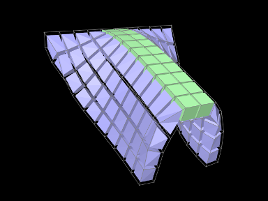
A simple model demonstrating the use of material bundles is defined in
artisynth.demos.tutorial.MaterialBundleDemo
It consists of a simple thin hexahedral sheet in which a material bundle is used to stiffen elements close to the x-axis, creating a stiff “spine”. While the same effect could be achieved by simply setting a different material property for the “spine” elements, it does provide a good example of material bundle usage. The model’s build method is given below:
Lines 6-9 create a thin FEM hex sheet, centered on the origin, with
size ![]() and
and ![]() elements
along each axis. Its material is set to a linear material with a
Young’s modulus of
elements
along each axis. Its material is set to a linear material with a
Young’s modulus of ![]() . The leftmost nodes are then fixed (lines
11-16).
. The leftmost nodes are then fixed (lines
11-16).
Next, a MaterialBundle is added and used to apply an additional
material to the elements near the x axis (lines 19-29). It is given a
neo-hookean material with a much higher stiffness, and the “spine”
elements for it are selected by finding those whose centroids
have a ![]() value within 0.1 of the x axis.
value within 0.1 of the x axis.
After the bundle is added, a control panel is created allowing interactive control of the materials for both the FEM model and the bundle, along with their elementWidgetSize properties.
Finally, some render properties are set (lines 41-44). The idea is to render the elements of both the FEM model and the bundle using element widgets (both of which will be visible since there is no surface rendering and the element widget sizes for both are greater than 0). The widget size for the bundle is made larger than that of the FEM model to ensure its widgets will cover those of the latter. Widget colors are controlled by the FEM and bundle face colors, set in lines 41-42.
The example can be run in ArtiSynth by selecting All demos > tutorial > MaterialBundleDemo from the Models menu. When it is run, the sheet will fall under gravity but be much stiffer along the spine (Figure 6.15). The control panel can be used to interactively adjust the material parameters for both the FEM and the bundle. This is one advantage of using bundles: the same material can be used to control multiple elements. The panel also allows interactive adjustment of the widget sizes, to illustrate what they look like and how they are rendered.
6.9 Muscle activated FEM models
Finite element muscle models are an extension to regular FEM models. As such, everything previously discussed for regular FEM models also applies to FEM muscles. Muscles have additional properties that allow them to contract when activated. There are two types of muscles supported:
- Fibre-based:
-
Point-to-point muscle fibres are embedded in the model.
- Material-based:
-
An auxiliary material is added to the constitutive law to embed muscle properties.
In this section, both types will be described.
6.9.1 FemMuscleModel
The main class for FEM-based muscles is FemMuscleModel, a subclass of FemModel3d. It differs from a basic FEM model in that it has the new property
| Property | Description |
| muscleMaterial | An object that adds an activation-dependent ‘muscle’ term to the constitutive law. |
This is a delegate object of type MuscleMaterial, described in detail in Section 6.10.3, that computes activation-dependent stress and stiffness in the muscle. In addition to this property, FemMuscleModel adds two new lists of subcomponents:
- bundles
-
Groupings of muscle sub-units (fibres or elements) that can be activated. - exciters
-
Components that control the activation of a set of bundles or other exciters.
6.9.1.1 Bundles
Muscle bundles allow for a muscle to be partitioned into separate groupings of fibres/elements, where each bundle can be activated independently. They are implemented in the class MuscleBundle. Bundles have three key properties:
| Property | Description |
|---|---|
| excitation | Activation level of the muscle, |
| fibresActive | Enable/disable “fibre-based” muscle components. |
| muscleMaterial | An object that adds an activation-dependent ‘muscle’ term to the constitutive law (Section 6.10.3). |
The excitation property controls the level of muscle activation, with zero being no muscle action, and one being fully activated. The fibresActive property is a boolean variable that controls whether or not to treat any contained fibres as point-to-point-like muscles (“fibre-based”). If false, the fibres are ignored. The third property, muscleMaterial, allows for a MuscleMaterial to be specified per bundle. By default, its value is inherited from FemMuscleModel.
6.9.1.2 Exciters
A MuscleExciter component enables you to simultaneously activate a group of “excitation components”. This includes: point-to-point muscles, muscle bundles, muscle fibres, material-based muscle elements, and other muscle exciters. Components that can be excited all implement the ExcitationComponent interface. To add or remove a component to the exciter, use
If a gain factor is specified, the activation is scaled by the gain for that component.
6.9.2 Fibre-based muscles
In fibre-based muscles, a set of point-to-point muscle fibres are added between FEM nodes or markers. Each fibre is assigned an AxialMuscleMaterial, just like for regular point-to-point muscles (Section 4.5.1). Note that these muscle materials typically have a “rest length” property, that will likely need to be adjusted for each fibre. Once the set of fibres are added to a MuscleBundle, they need to be enabled. This is done by setting the fibresActive property of the bundle to true.
Fibres are added to a MuscleBundle using one of the functions:
The latter returns the newly created Muscle fibre. The following code snippet demonstrates how to create a fibre-based MuscleBundle and add it to an FEM muscle.
In these fibre-based muscles, force is only exerted between the anchor points of the fibres; it is a discrete approximation. These models are typically more stable than material-based ones.
6.9.3 Material-based muscles
In material-based muscles, the constitutive law is augmented with additional terms to account for muscle-specific properties. This is a continuous representation within the model.
The basic building block for a material-based muscle bundle is a MuscleElementDesc. This object contains a reference to a FemElement3d, a MuscleMaterial, and either a single direction or set of directions that specify the direction of contraction. If a single direction is specified, then it is assumed the entire element contracts in the same direction. Otherwise, a direction can be specified for each integration point within the element. A null direction signals that there is no muscle at the corresponding point. This allows for a sub-element resolution for muscle definitions. The positions of integration points for a given element can be obtained with:
By default, the MuscleMaterial is inherited from the bundle’s material property. Muscle materials are described in detail in Section 6.10.3 and include GenericMuscle, BlemkerMuscle, and FullBlemkerMuscle. The Blemker-type materials are based on [5].
Elements can be added to a muscle bundle using one of the methods:
The following snippet demonstrates how to create and add a material-based muscle bundle:
6.9.4 Example: toy FEM muscle model
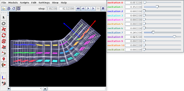
A simple example showing an FEM with material-based muscles is given by artisynth.demos.tutorial.ToyMuscleFem. It consists of a hex-element beam, with 12 muscles added in groups along its length, allowing it to flex in the x-z plane. A frame object is also attached to the right end. The code for the model, without the package and import directives, is listed below:
Within the build() method, the mech model is created in the usual way (lines 8-10). Gravity is turned off to give the muscles greater control over the FEM model’s configuration. The MechModel reference is stored in the class field myMech to enable any subclasses to have easy access to it; the same will be done for the FEM model and the attached frame.
The FEM model itself is created at lines (12-24). An instance of FemMuscleModel is created and then passed to FemFactory.createHexGrid(); this allows the model to be an instance of FemMuscleModel instead of FemModel3d. The model is assigned a linear material with Poisson’s ratio of 0 to allow it to be easily compressed. Muscle bundles will be material-based and will all use the same SimpleForceMuscle material that is assigned to the model’s muscleMaterial property. Density and damping parameters are defined so as to improve model stability when muscles are excited. Once the model is created, its left-hand nodes are fixed to provide anchoring (lines 27-32).
Muscle bundles are created at lines 36-58. There are 12 of them, arranged in three vertical layers and four horizontal sections. Each bundle is populated with 9 adjacent elements in the x-y plane. To find these elements, their center positions are calculated and then passed to the FEM method findNearestVolumetricElement(). The element is then added to the bundle with a resting activation direction parallel to the x axis. For visualization, each bundle’s line color is set to a distinct color from the numeric probe display palette, based on the bundle’s number (lines 53-54).
After the bundles have been added to the FEM model, a control is created to allow interactive control of their excitations (lines 88-95). Each widget is labeled excitation N, where N is the bundle number, and the label is colored to match the bundle’s line color. Finally, a frame is created and attached to the FEM model (lines 59-62), and render properties are set at lines 106-115: Muscle bundles are drawn by showing the activation direction in each element; the frame is displayed as a solid arrow with axis lengths of 0.3; the FEM line and face colors are set to blue-gray, and the surface is rendered and made transparent.
To run this example in ArtiSynth, select All demos > tutorial > ToyMuscleFem from the Models menu. Running the model and adjusting the exciters in the control panel will cause the FEM model to deform in various ways (Figure 6.16).
6.9.5 Example: comparison with two beam examples
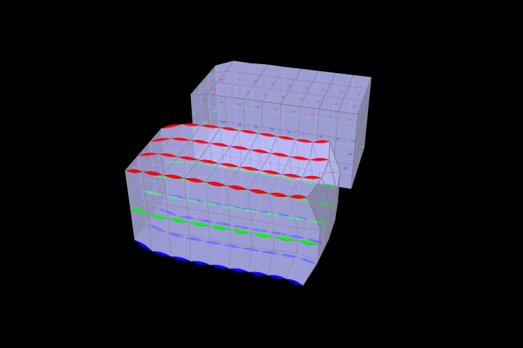
An example comparing a fibre-based and a material-based muscle is shown in Figure 6.17. The code can be found in artisynth.demos.tutorial.FemMuscleBeams. There are two FemMuscleModel beams in the model: one fibre-based, and one material-based. Each has three muscle bundles: one at the top (red), one in the middle (green), and one at the bottom (blue). In the figure, both muscles are fully activated. Note the deformed shape of the beams. In the fibre-based one, since forces only act between point on the fibres, the muscle seems to bulge. In the material-based muscle, the entire continuous volume contracts, leading to a uniform deformation.
Material-based muscles are more realistic. However, this often comes at the cost of stability. The added terms to the constitutive law are highly nonlinear, which may cause numerical issues as elements become highly contracted or highly deformed. Fibre-based muscles are, in general, more stable. However, they can lead to bulging and other deformation artifacts due to their discrete nature.
6.10 Material types
ArtiSynth FEM models support a variety of material types, including
linear, hyperelastic, and activated muscle materials, described in the
sections below. These can be used to supply the primary material for
either an entire FEM model or for specific elements (using the setMaterial() methods for either). They can also be used to supply
auxiliary materials, whose behavior is superimposed on the underlying
material, via either material bundles
(Section 6.8) or,
for FemMuscleModels, muscle bundles
(Section 6.9). Many of the properties for a given
material can be bound to a scalar or vector field
(Section 7.2) to allow their values to vary across an
FEM model. In the descriptions below, properties for which this is
true will have a ![]() indicated under the “Field” entry in the
material’s property table.
indicated under the “Field” entry in the
material’s property table.
All materials are defined in the package artisynth.core.materials.
6.10.1 Linear
Linear materials determine Cauchy stress ![]() as a linear mapping
from the small deformation Cauchy strain
as a linear mapping
from the small deformation Cauchy strain ![]() ,
,
| (6.7) |
where ![]() is the elasticity tensor.
Both the stress and
strain are symmetric
is the elasticity tensor.
Both the stress and
strain are symmetric ![]() matrices,
matrices,
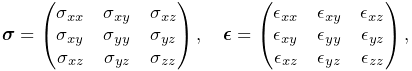 |
(6.8) |
and can be expressed as 6-vectors using Voigt notation:
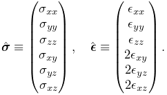 |
(6.9) |
This allows the constitutive mapping to be expressed in matrix form as
| (6.10) |
where ![]() is the
is the ![]() elasticity matrix.
elasticity matrix.
Different Voigt notation mappings appear in the literature with regard to off-diagonal matrix entries. We use the one employed by FEBio [13]. Another common mapping is
Traditionally, Cauchy strain is computed from the symmetric part of
the deformation gradient ![]() using the formula
using the formula
| (6.11) |
where ![]() is the
is the ![]() identity matrix. However, ArtiSynth
materials support corotation, in which rotations are first
removed from
identity matrix. However, ArtiSynth
materials support corotation, in which rotations are first
removed from ![]() using a polar decomposition
using a polar decomposition
| (6.12) |
where ![]() is a (right-handed) rotation matrix and
is a (right-handed) rotation matrix and ![]() is a symmetric
matrix.
is a symmetric
matrix. ![]() is then used to compute the Cauchy strain:
is then used to compute the Cauchy strain:
| (6.13) |
Corotation is the default behavior for linear materials in ArtiSynth and allows models to handle large scale rotational deformations [18, 16].
For linear materials, the stress/strain response is computed at a single integration point in the center of each element. This is done
to improve computational efficiency, as it allows the precomputation
of stiffness matrices that map nodal displacements onto nodal forces
for each element. This precomputed matrix can then be adjusted during
each simulation step to account for the rotation ![]() computed at each
element’s integration
point [18, 16].
computed at each
element’s integration
point [18, 16].
Specific linear material types are listed in the subsections below. All are subclasses of LinearMaterialBase, and in addition to their individual properties, all export a corotation property (default value true) that controls whether corotation is applied.
6.10.1.1 LinearMaterial
LinearMaterial is a standard isotropic linear material, which is also the default material for FEM models. Its elasticity matrix is given by
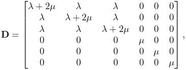 |
(6.14) |
where the Lamé parameters ![]() and
and ![]() are
derived from Young’s modulus
are
derived from Young’s modulus ![]() and Poisson’s ratio
and Poisson’s ratio ![]() via
via
| (6.15) |
The material behavior is controlled by the following properties:
| Property | Description | Default | Field | |
|---|---|---|---|---|
| YoungsModulus | Young’s modulus | 500000 | ✓ | |
| PoissonsRatio | Poisson’s ratio | 0.33 | ||
| corotated | applies corotation if true | true |
LinearMaterials can be created with the following constructors:
| LinearMaterial() |
Create with default properties. |
| LinearMaterial (double E, double nu) |
Create with specified |
| LinearMaterial (double E, double nu, boolean corotated) |
Create with specified |
6.10.1.2 TransverseLinearMaterial
TransverseLinearMaterial
is a transversely isotropic linear material whose behavior is
symmetric about a prescribed polar axis. If the polar axis is
parallel to the ![]() axis, then the elasticity matrix is specified most
easily in terms of its inverse, or compliance matrix, according
to
axis, then the elasticity matrix is specified most
easily in terms of its inverse, or compliance matrix, according
to
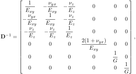 |
where ![]() and
and ![]() are Young’s moduli transverse
and parallel to the axis, respectively,
are Young’s moduli transverse
and parallel to the axis, respectively, ![]() and
and ![]() are
Poisson’s ratios transverse and parallel to the axis, and
are
Poisson’s ratios transverse and parallel to the axis, and ![]() is the
shear modulus.
is the
shear modulus.
The material behavior is controlled by the following properties:
| Property | Description | Default | Field | |
|---|---|---|---|---|
| youngsModulus | Young’s moduli transverse and parallel to the axis | ✓ | ||
| poissonsRatio | Poisson’s ratios transverse and parallel to the axis | |||
| shearModulus | shear modulus | 187970 | ✓ | |
| direction | direction of the polar axis | ✓ | ||
| corotated | applies corotation if true | true |
The youngsModulus and poissonsRatio properties are both described by Vector2d objects, while direction is described by a Vector3d. The direction property (as well as youngsModulus and shearModulus) can be bound to a field to allow its value to vary over an FEM model (Section 7.2).
TransverseLinearMaterials can be created with the following constructors:
| TransverseLinearMaterial() |
Create with default properties. |
| TransverseLinearMaterial (Vector2d E, double G, Vector2d nu, boolean corotated) |
Create with specified |
6.10.1.3 AnisotropicLinearMaterial
AnisotropicLinearMaterial
is a general anisotropic linear material whose behavior is specified
by an arbitrary (symmetric) elasticity matrix ![]() .
The material behavior is controlled by the following properties:
.
The material behavior is controlled by the following properties:
| Property | Description | Default | Field | |
|---|---|---|---|---|
| stiffnessTensor | symmetric |
|||
| corotated | applies corotation if true | true |
The default value for stiffnessTensor is an isotropic elasticity
matrix corresponding to ![]() and
and ![]() .
.
AnisotropicLinearMaterials can be created with the following constructors:
| AnisotropicLinearMaterial() |
Create with default properties. |
| AnisotropicLinearMaterial (Matrix6dBase D) |
Create with specified elasticity |
| AnisotropicLinearMaterial (Matrix6dBase D, boolean corotated) |
Create with specified |
6.10.2 Hyperelastic materials
A hyperelastic material is defined by a strain energy density
function ![]() that is in general a function of the deformation gradient
that is in general a function of the deformation gradient
![]() , and more specifically a quantity derived from
, and more specifically a quantity derived from ![]() that is
rotationally invariant, such as the right Cauchy Green
tensor
that is
rotationally invariant, such as the right Cauchy Green
tensor ![]() , the left Cauchy Green
tensor
, the left Cauchy Green
tensor ![]() , or Green strain
, or Green strain
| (6.15) |
![]() is often described with respect to the first or second invariants
of these quantities, denoted by
is often described with respect to the first or second invariants
of these quantities, denoted by ![]() and
and ![]() and defined with
respect to a given matrix
and defined with
respect to a given matrix ![]() by
by
| (6.16) |
Alternatively, ![]() is sometimes defined with respect to the three
principal stretches of the deformation,
is sometimes defined with respect to the three
principal stretches of the deformation, ![]() , which are the eigenvalues of the symmetric component
, which are the eigenvalues of the symmetric component ![]() of the
polar decomposition of
of the
polar decomposition of ![]() in (6.12).
in (6.12).
If ![]() is expressed with respect to
is expressed with respect to ![]() , then the second
Piola-Kirchhoff stress
, then the second
Piola-Kirchhoff stress ![]() is given by
is given by
| (6.17) |
from which the Cauchy stress can be obtained via
| (6.18) |
Many of the hyperelastic materials described below are incompressible, in the sense that ![]() is partitioned into a deviatoric component that is volume invariant and a dilational
component that depends solely on volume changes.
Volume change is
characterized by
is partitioned into a deviatoric component that is volume invariant and a dilational
component that depends solely on volume changes.
Volume change is
characterized by ![]() , with the change in volume given by
, with the change in volume given by ![]() and
and ![]() indicating no volume change. Deviatoric
changes are characterized by
indicating no volume change. Deviatoric
changes are characterized by ![]() , with
, with
| (6.19) |
and so the partitioned strain energy density function assumes the form
| (6.20) |
where the ![]() term is the deviatoric contribution and
term is the deviatoric contribution and
![]() is the volumetric potential that enforces incompressibility.
is the volumetric potential that enforces incompressibility.
![]() may also be expressed with respect to the right deviatoric
Cauchy Green tensor
may also be expressed with respect to the right deviatoric
Cauchy Green tensor ![]() or the left deviatoric Cauchy Green
tensor
or the left deviatoric Cauchy Green
tensor ![]() , respectively defined by
, respectively defined by
| (6.21) |
ArtiSynth supplies different forms of ![]() , as specified by a
material’s bulkPotential property and detailed in
Section 6.7.3. All of the available potentials depend
on a bulkModulus property
, as specified by a
material’s bulkPotential property and detailed in
Section 6.7.3. All of the available potentials depend
on a bulkModulus property ![]() , and so
, and so ![]() is often
expressed as
is often
expressed as ![]() . A larger bulk modulus will make the
material more incompressible, with effective incompressibility
typically achieved by setting
. A larger bulk modulus will make the
material more incompressible, with effective incompressibility
typically achieved by setting ![]() to a value that exceeds the
other elastic moduli in the material by a factor of 100 or more.
All incompressible materials are subclasses of
IncompressibleMaterialBase.
to a value that exceeds the
other elastic moduli in the material by a factor of 100 or more.
All incompressible materials are subclasses of
IncompressibleMaterialBase.
6.10.2.1 St Venant-Kirchoff material
StVenantKirchoffMaterial
is a compressible isotropic material that extends isotropic linear
elasticity to large deformations.
The strain energy density is most easily expressed as a function
of the Green strain ![]() :
:
| (6.22) |
where the Lamé parameters ![]() and
and ![]() are
derived from Young’s modulus
are
derived from Young’s modulus ![]() and Poisson’s ratio
and Poisson’s ratio ![]() according to (6.15).
From this definition it follows that the second Piola-Kirchhoff stress
tensor is given by
according to (6.15).
From this definition it follows that the second Piola-Kirchhoff stress
tensor is given by
| (6.23) |
The material behavior is controlled by the following properties:
| Property | Description | Default | Field | |
|---|---|---|---|---|
| YoungsModulus | Young’s modulus | 500000 | ✓ | |
| PoissonsRatio | Poisson’s ratio | 0.33 |
StVenantKirchoffMaterials can be created with the following constructors:
| StVenantKirchoffMaterial() |
Create with default properties. |
| StVenantKirchoffMaterial (double E, double nu) |
Create with specified elasticity |
6.10.2.2 Neo-Hookean material
NeoHookeanMaterial
is a compressible isotropic material with a strain energy density
expressed as a function of the first invariant ![]() of the right
Cauchy-Green tensor
of the right
Cauchy-Green tensor ![]() and
and ![]() :
:
| (6.23) |
where the Lamé parameters ![]() and
and ![]() are derived from
Young’s modulus
are derived from
Young’s modulus ![]() and Poisson’s ratio
and Poisson’s ratio ![]() via
(6.15). The Cauchy stress can be expressed in terms of
the left Cauchy-Green tensor
via
(6.15). The Cauchy stress can be expressed in terms of
the left Cauchy-Green tensor ![]() as
as
| (6.24) |
The material behavior is controlled by the following properties:
| Property | Description | Default | Field | |
|---|---|---|---|---|
| YoungsModulus | Young’s modulus | 500000 | ✓ | |
| PoissonsRatio | Poisson’s ratio | 0.33 |
NeoHookeanMaterials can be created with the following constructors:
| NeoHookeanMaterial() |
Create with default properties. |
| NeoHookeanMaterial (double E, double nu) |
Create with specified elasticity |
6.10.2.3 Incompressible neo-Hookean material
IncompNeoHookeanMaterial
is an incompressible version of the neo-Hookean material,
with a strain energy density expressed in terms of the
first invariant ![]() of the deviatoric
right Cauchy-Green tensor
of the deviatoric
right Cauchy-Green tensor ![]() , plus a potential
function
, plus a potential
function ![]() to enforce incompressibility:
to enforce incompressibility:
| (6.24) |
The material behavior is controlled by the following properties:
| Property | Description | Default | Field | |
|---|---|---|---|---|
| shearModulus | shear modulus | 150000 | ✓ | |
| bulkModulus | bulk modulus for incompressibility | 100000 | ✓ | |
| bulkPotential | incompressibility potential function |
QUADRATIC |
IncompNeoHookeanMaterials can be created with the following constructors:
| IncompNeoHookeanMaterial() |
Create with default properties. |
| IncompNeoHookeanMaterial (double G, double kappa) |
Create with specified elasticity |
6.10.2.4 Mooney-Rivlin material
MooneyRivlinMaterial
is an incompressible isotropic material with a strain energy density
expressed as a polynomial of the first and second invariants ![]() and
and ![]() of the right deviatoric Cauchy-Green
tensor
of the right deviatoric Cauchy-Green
tensor ![]() . ArtiSynth supplies a five parameter version of this
model, with a strain energy density given by
. ArtiSynth supplies a five parameter version of this
model, with a strain energy density given by
| (6.24) |
A two-parameter version (![]() ,
, ![]() ) is often found in the
literature, consisting of only the first two terms:
) is often found in the
literature, consisting of only the first two terms:
| (6.25) |
The material behavior is controlled by the following properties:
| Property | Description | Default | Field | |
|---|---|---|---|---|
| C10 | first coefficient | 150000 | ✓ | |
| C01 | second coefficient | 0 | ✓ | |
| C11 | third coefficient | 0 | ✓ | |
| C20 | fourth coefficient | 0 | ✓ | |
| C02 | fifth coefficient | 0 | ✓ | |
| bulkModulus | bulk modulus for incompressibility | 100000 | ✓ | |
| bulkPotential | incompressibility potential function |
QUADRATIC |
MooneyRivlinMaterials can be created with the following constructors:
| MooneyRivlinMaterial() |
Create with default properties. |
| MooneyRivlinMaterial (double C10, double C01, double C11, double C20, double C02, double kappa) |
Create with specified coefficients. |
6.10.2.5 Ogden material
OgdenMaterial
is an incompressible material with a strain energy density
expressed as a function of the deviatoric principal stretches ![]() :
:
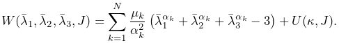 |
(6.25) |
ArtiSynth allows a maximum of six terms, corresponding to ![]() , and
the material behavior is controlled by the following properties:
, and
the material behavior is controlled by the following properties:
| Property | Description | Default | Field | |
|---|---|---|---|---|
| Mu1 | first multiplier | 300000 | ✓ | |
| Mu2 | second multiplier | 0 | ✓ | |
| ... | ... | ... | 0 | ✓ |
| Mu6 | final multiplier | 0 | ✓ | |
| Alpha1 | first multiplier | 2 | ✓ | |
| Alpha2 | second multiplier | 2 | ✓ | |
| ... | ... | ... | 2 | ✓ |
| Alpha6 | final multiplier | 2 | ✓ | |
| bulkModulus | bulk modulus for incompressibility | 100000 | ✓ | |
| bulkPotential | incompressibility potential function |
QUADRATIC |
OgdenMaterials can be created with the following constructors:
| OgdenMaterial() |
Create with default properties. |
| OgdenMaterial (double[] mu, double[] alpha, double kappa) |
Create with specified |
6.10.2.6 Fung orthotropic material
FungOrthotropicMaterial
is an incompressible orthotropic material defined with respect to an
![]() -
-![]() -
-![]() coordinate system expressed by a
coordinate system expressed by a ![]() rotation
matrix
rotation
matrix ![]() . The strain energy density is expressed as a function of
the deviatoric Green strain
. The strain energy density is expressed as a function of
the deviatoric Green strain
| (6.25) |
and the three unit direction vectors ![]() representing the columns of
representing the columns of ![]() . Letting
. Letting ![]() and defining
and defining
| (6.26) |
the energy density is given by
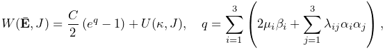 |
(6.27) |
where ![]() is a material coefficient and
is a material coefficient and ![]() and
and ![]() are
the orthotropic Lamé parameters.
are
the orthotropic Lamé parameters.
At present, the coordinate frame ![]() is not defined in the material,
but can be specified on a per-element basis using the element method
setFrame(Matrix3dBase). For example:
is not defined in the material,
but can be specified on a per-element basis using the element method
setFrame(Matrix3dBase). For example:
One should be careful to ensure that the argument to setFrame() is in fact an orthogonal rotation matrix as this will not be otherwise enforced.
The material behavior is controlled by the following properties:
| Property | Description | Default | Field | |
|---|---|---|---|---|
| mu1 | second Lamé parameter along |
1000 | ✓ | |
| mu2 | second Lamé parameter along |
1000 | ✓ | |
| mu3 | second Lamé parameter along |
1000 | ✓ | |
| lam11 | first Lamé parameter along |
2000 | ✓ | |
| lam22 | first Lamé parameter along |
2000 | ✓ | |
| lam33 | first Lamé parameter along |
2000 | ✓ | |
| lam12 | first Lamé parameter for |
2000 | ✓ | |
| lam23 | first Lamé parameter for |
2000 | ✓ | |
| lam31 | first Lamé parameter for |
2000 | ✓ | |
| C | C coefficient | 1500 | ✓ | |
| bulkModulus | bulk modulus for incompressibility | 100000 | ✓ | |
| bulkPotential | incompressibility potential function |
QUADRATIC |
FungOrthotropicMaterials can be created with the following constructors:
| FungOrthotropicMaterial() |
Create with default properties. |
| FungOrthotropicMaterial (double mu1, double mu2, double mu3, double lam11, double lam22, double lam33, double lam12, double lam23, double lam31, double C, double kappa) |
Create with specified properties. |
6.10.2.7 Yeoh material
YeohMaterial is an incompressible isotropic material that implements a Yeoh model with a strain energy density containing up to five terms:
 |
(6.27) |
where ![]() is the first invariant of the right deviatoric Cauchy Green
tensor and
is the first invariant of the right deviatoric Cauchy Green
tensor and ![]() are the material coefficients.
The material behavior is controlled by the following properties:
are the material coefficients.
The material behavior is controlled by the following properties:
| Property | Description | Default | Field | |
|---|---|---|---|---|
| C1 | first coefficient (shear modulus) | 150000 | ✓ | |
| C2 | second coefficient | 0 | ✓ | |
| C3 | third coefficient | 0 | ✓ | |
| C4 | fourth coefficient | 0 | ✓ | |
| C5 | fifth coefficient | 0 | ✓ | |
| bulkModulus | bulk modulus for incompressibility | 100000 | ✓ | |
| bulkPotential | incompressibility potential function |
QUADRATIC |
YeohMaterials can be created with the following constructors:
| YeohMaterial() |
Create with default properties. |
| YeohMaterial (double C1, double C2, double C3, double kappa) |
Create three term material with |
| YeohMaterial (double C1, double C2, double C3, double C4, double C5, double kappa) |
Create five term material with |
6.10.2.8 Arruda-Boyce material
ArrudaBoyceMaterial is an incompressible isotropic material that implements the Arruda-Boyce model [2]. Its strain energy density is given by
 |
(6.27) |
where ![]() is the initial modulus,
is the initial modulus, ![]() the
locking stretch,
the
locking stretch, ![]() the first invariant of the
right deviatoric Cauchy Green tensor, and
the first invariant of the
right deviatoric Cauchy Green tensor, and
The material behavior is controlled by the following properties:
| Property | Description | Default | Field | |
|---|---|---|---|---|
| mu | initial modulus | 1000 | ✓ | |
| lambdaMax | locking stretch | 2.0 | ✓ | |
| bulkModulus | bulk modulus for incompressibility | 100000 | ✓ | |
| bulkPotential | incompressibility potential function |
QUADRATIC |
ArrudaBoyceMaterials can be created with the following constructors:
| ArrudaBoyceMaterial() |
Create with default properties. |
| ArrudaBoyceMaterial (double mu, double lmax, double kappa) |
Create with specified |
6.10.2.9 Veronda-Westmann material
VerondaWestmannMaterial is an incompressible isotropic material that implements the Veronda-Westmann model [28]. Its strain energy density is given by
| (6.28) |
where ![]() and
and ![]() are material coefficients and
are material coefficients and ![]() and
and
![]() the first and second invariants of the right deviatoric
Cauchy Green tensor.
the first and second invariants of the right deviatoric
Cauchy Green tensor.
The material behavior is controlled by the following properties:
| Property | Description | Default | Field | |
|---|---|---|---|---|
| C1 | first coefficient | 1000 | ✓ | |
| C2 | second coefficient | 10 | ✓ | |
| bulkModulus | bulk modulus for incompressibility | 100000 | ✓ | |
| bulkPotential | incompressibility potential function |
QUADRATIC |
VerondaWestmannMaterials can be created with the following constructors:
| VerondaWestmannMaterial() |
Create with default properties. |
| VerondaWestmannMaterial (double C1, double C2, double kappa) |
Create with specified |
6.10.2.10 Incompressible material
IncompressibleMaterial is an incompressible isotropic material that implements pure incompressibility, with an energy density function given by
| (6.28) |
Because it responds only to dilational strains, it must be used in conjunction with another material to resist deviatoric strains. In this context, it can be used to provide dilational support to deviatoric-only materials such as the FullBlemkerMuscle (Section 6.10.3.3).
The material behavior is controlled by the following properties:
| Property | Description | Default | Field | |
|---|---|---|---|---|
| bulkModulus | bulk modulus for incompressibility | 100000 | ✓ | |
| bulkPotential | incompressibility potential function |
QUADRATIC |
IncompressibleMaterials can be created with the following constructors:
| IncompressibleMaterial() |
Create with default values. |
| IncompressibleMaterial (double kappa) |
Create with specified |
6.10.3 Muscle materials
Muscle materials are used to exert stress along a particular direction within a material. This stress may contain both an active component, which depends on the muscle excitation, and a passive component, which depends solely on the stretch along the prescribed direction. Because most muscle materials act only along one direction, they are typically deployed within an FEM as additional materials that act in addition to an underlying material. This can be done using either muscle bundles within a FemMuscleModel (Section 6.9.1.1) or material bundles within any FEM model (Sections 6.8 and 7.5.2).
All of the muscle materials described below assume (near)
incompressibility, and so the directional stress is a function of the
deviatoric stretch ![]() along the muscle direction instead of the
overall stretch
along the muscle direction instead of the
overall stretch ![]() . The former can be determined from the
latter via
. The former can be determined from the
latter via
| (6.28) |
where ![]() is the determinant of the deformation gradient. The
directional Cauchy stress
is the determinant of the deformation gradient. The
directional Cauchy stress ![]() resulting from the material is
computed from
resulting from the material is
computed from
 |
(6.29) |
where ![]() is a force term,
is a force term, ![]() is a unit vector indicating
the current muscle direction in spatial coordinates, and
is a unit vector indicating
the current muscle direction in spatial coordinates, and ![]() is the
is the ![]() identity matrix. In a purely passive case when the force arises
from a stress energy density function
identity matrix. In a purely passive case when the force arises
from a stress energy density function ![]() , we have
, we have
| (6.30) |
The muscle direction is specified in one of two ways, depending on how
the muscle material is deployed. All muscle materials export a
property restDir which specifies the direction in material
(rest) coordinates. It has a default value of ![]() , and can
be either set explicitly or bound to a field to allow it to vary over the
entire model (Section 7.5.2). However, if a muscle
material is deployed within a muscle bundle
(Section 6.9.1), then the restDir property is
ignored and the direction is instead specified by the
MuscleElementDesc components contained
within the bundle (Section 6.9.3).
, and can
be either set explicitly or bound to a field to allow it to vary over the
entire model (Section 7.5.2). However, if a muscle
material is deployed within a muscle bundle
(Section 6.9.1), then the restDir property is
ignored and the direction is instead specified by the
MuscleElementDesc components contained
within the bundle (Section 6.9.3).
Likewise, muscle excitation is specified using the material’s excitation property, unless the material is deployed within a muscle bundle, in which case it is controlled by the excitation property of the bundle.
6.10.3.1 Generic muscle
GenericMuscle
is a muscle material whose force term ![]() is given by
is given by
| (6.31) |
where ![]() is the excitation signal,
is the excitation signal, ![]() is a maximum stress
term, and
is a maximum stress
term, and ![]() is a passive force given by
is a passive force given by
 |
(6.32) |
In the equation above, ![]() is the exponential stress coefficient,
is the exponential stress coefficient,
![]() is the uncrimping factor, and
is the uncrimping factor, and ![]() and
and ![]() are computed to
provide
are computed to
provide ![]() continuity at
continuity at ![]() .
.
The material behavior is controlled by the following properties:
| Property | Description | Default | Field | |
|---|---|---|---|---|
| maxStress | maximum stress | 30000 | ✓ | |
| maxLambda |
|
1.4 | ✓ | |
| expStressCoeff | exponential stress coefficient | 0.05 | ✓ | |
| uncrimpingFactor | uncrimping factor | 6.6 | ✓ | |
| restDir | direction in material coordinates | ✓ | ||
| excitation | activation signal | 0 |
GenericMuscles can be created with the following constructors:
| GenericMuscle() |
Create with default values. |
| GenericMuscle (double maxLambda, double maxStress, double expStressCoef, double uncrimpFactor) |
Create with specified |
The constructors do not specify restDir. If the material is not being deployed within a muscle bundle, then restDir should also be set appropriately, either directly or via a field (Section 7.5.2).
6.10.3.2 Blemker muscle
BlemkerMuscle
is a muscle material implementing the directional component of the
model proposed by Sylvia Blemker [5]. Its force
term ![]() is given by
is given by
| (6.32) |
where ![]() is a maximum stress term,
is a maximum stress term, ![]() is the excitation
signal,
is the excitation
signal, ![]() is an active force-length curve, and
is an active force-length curve, and ![]() is
the passive force.
is
the passive force. ![]() and
and ![]() are described in
terms of
are described in
terms of ![]() :
:
 |
(6.33) |
and
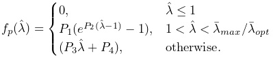 |
(6.34) |
In the equation for ![]() ,
, ![]() is the exponential stress
coefficient,
is the exponential stress
coefficient, ![]() is the uncrimping factor, and
is the uncrimping factor, and ![]() and
and ![]() are
computed to provide
are
computed to provide ![]() continuity at
continuity at ![]() .
.
The material behavior is controlled by the following properties:
| Property | Description | Default | Field | |
|---|---|---|---|---|
| maxStress | maximum stress | 300000 | ✓ | |
| optLambda |
|
1 | ✓ | |
| maxLambda |
|
1.4 | ✓ | |
| expStressCoeff | exponential stress coefficient | 0.05 | ✓ | |
| uncrimpingFactor | uncrimping factor | 6.6 | ✓ | |
| restDir | direction in material coordinates | ✓ | ||
| excitation | activation signal | 0 |
BlemkerMuscles can be created with the following constructors:
| BlemkerMuscle() |
Create with default values. |
| BlemkerMuscle (double maxLam, double optLam, double maxStress, double expStressCoef, double uncrimpFactor) |
Create with specified |
The constructors do not specify restDir. If the material is not being deployed within a muscle bundle, then restDir should also be set appropriately, either directly or via a field (Section 7.5.2).
6.10.3.3 Full Blemker muscle
FullBlemkerMuscle
is a muscle material implementing the entire model proposed by Sylvia
Blemker [5]. This includes the directional
stress described in Section 6.10.3.2, plus additional
passive terms to model the tissue material matrix. The latter is based
on a strain energy density function ![]() given by
given by
| (6.34) |
where ![]() and
and ![]() are the along-fibre and cross-fibre
shear moduli, respectively, and
are the along-fibre and cross-fibre
shear moduli, respectively, and ![]() and
and ![]() are
Criscione invariants. The latter are defined as follows: Let
are
Criscione invariants. The latter are defined as follows: Let ![]() and
and ![]() be the invariants of the deviatoric left Cauchy
Green tensor
be the invariants of the deviatoric left Cauchy
Green tensor ![]() ,
, ![]() the unit vector giving the current muscle
direction in spatial coordinates, and
the unit vector giving the current muscle
direction in spatial coordinates, and ![]() and
and ![]() additional invariants defined by
additional invariants defined by
| (6.35) |
Then, defining
 |
![]() and
and ![]() are given by
are given by
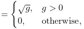 |
(6.36) | |||
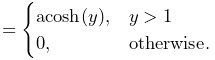 |
(6.37) |
At present, FullBlemkerMuscle does not implement a volumetric potential function
. That means it responds solely to deviatoric strains, and so if it is being used as a model’s primary material, it should be augmented with an additional material to provide resistance to compression. A simple choice for this is the purely incompressible material IncompressibleMaterial, described in Section 6.10.2.10.
The material behavior is controlled by the following properties:
| Property | Description | Default | Field | |
|---|---|---|---|---|
| maxStress | maximum stress | 300000 | ✓ | |
| optLambda |
|
1 | ✓ | |
| maxLambda |
|
1.4 | ✓ | |
| expStressCoeff | exponential stress coefficient | 0.05 | ✓ | |
| uncrimpingFactor | uncrimping factor | 6.6 | ✓ | |
| G1 | along-fibre shear modulus | 0 | ✓ | |
| G2 | cross-fibre shear modulus | 0 | ✓ | |
| restDir | direction in material coordinates | ✓ | ||
| excitation | activation signal | 0 |
FullBlemkerMuscles can be created with the following constructors:
| FullBlemkerMuscle() |
Create with default values. |
| BlemkerMuscle (double maxLam, double optLam, double maxStress, double expStressCoef, double uncrimpFactor, double G1, double G2) |
Create with |
The constructors do not specify restDir. If the material is not being deployed within a muscle bundle, then restDir should also be set appropriately, either directly or via a field (Section 7.5.2).
6.10.3.4 Simple force muscle
SimpleForceMuscle
is a very simple muscle material whose force term ![]() is
given by
is
given by
| (6.38) |
where ![]() is the excitation signal and
is the excitation signal and ![]() is a maximum
stress term. It can be useful as a debugging tool.
is a maximum
stress term. It can be useful as a debugging tool.
The material behavior is controlled by the following properties:
| Property | Description | Default | Field | |
|---|---|---|---|---|
| maxStress | maximum stress | 30000 | ✓ | |
| restDir | direction in material coordinates | ✓ | ||
| excitation | activation signal | 0 |
SimpleForceMuscles can be created with the following constructors:
| SimpleForceMuscle() |
Create with default values. |
| SimpleForceMuscle (double maxStress) |
Create with specified |
The constructors do not specify restDir. If the material is not being deployed within a muscle bundle, then restDir should also be set appropriately, either directly or via a field (Section 7.5.2).
6.11 Stress, strain and strain energy
An ArtiSynth FEM model has the capability to compute a variety of stress and strain measures at each of its nodes, as well as strain energy for each element and for the entire model.
6.11.1 Computing nodal values
Stress, strain, and strain energy density can be computed at each node of an FEM model. By default, these quantities are not computed, in order to conserve computing power. However, their computation can be enabled with the FemModel3d properties computeNodalStress, computeNodalStrain and computeNodalEnergyDensity, which can be set either in the GUI, or using the following accessor methods:
| void setComputeNodalStress(boolean) |
Enable stress to be computed at each node. |
| boolean getComputeNodalStress() |
Queries if nodal stress computation enabled. |
| void setComputeNodalStrain(boolean) |
Enable strain to be computed at each node. |
| boolean getComputeNodalStrain() |
Queries if nodal strain computation enabled. |
| void setComputeNodalEnergyDensity(boolean) |
Enable strain energy density to be computed at each node. |
| boolean getComputeNodalEnergyDensity() |
Queries if nodal strain energy density computation enabled. |
Setting these properties to true will cause their respective values to be computed at the nodes during each subsequent simulation step. This is done by computing values at the element integration points, extrapolating these values to the nodes, and then averaging them across the contributions from all surrounding elements.
Once computed, the values may be obtained at each node using the following FemNode3d methods:
| SymmetricMatrix3d getStress() |
Returns the current Cauchy stress at the node. |
| SymmetricMatrix3d getStrain() |
Returns the current strain at the node. |
| double getEnergyStrain() |
Returns the current strain energy density at the node. |
The stress value is the Cauchy stress. The strain values depend on the
primary material within each element: if the material is linear,
strain will be the small deformation Cauchy strain (co-rotated if the
material’s corotated property is true), while otherwise it
will be Green strain ![]() :
:
| (6.38) |
where ![]() is the right Cauchy-Green tensor.
is the right Cauchy-Green tensor.
6.11.2 Scalar stress/strain measures
Stress or strain values are tensor quantities represented by symmetric
![]() matrices. If they are being computed at the nodes, a
variety of scalar quantities can be extracted from them, using the
FemNode3d method
matrices. If they are being computed at the nodes, a
variety of scalar quantities can be extracted from them, using the
FemNode3d method
| double getStressStrainMeasure(StressStrainMeasure m) |
where StressStrainMeasure is an enumerated type with the following entries:
- VonMisesStress
-
von Mises stress, equal to

where
 the second invariant of the average deviatoric stress.
 - MAPStress
-
Absolute value of the maximum principle Cauchy stress.
- MaxShearStress
-
Maximum shear stress, given by

where
 ,
,  and
and  are the eigenvalues of the stress tensor.
 - VonMisesStrain
-
von Mises strain, equal to

where
the second invariant of the average deviatoric strain. - MAPStrain
-
Absolute value of the maximum principle strain.
- MaxShearStrain
-
Maximum shear strain, given by
where
, and are the eigenvalues of the strain tensor. - EnergyDensity
-
Strain energy density.
These quantities can also be queried with the following convenience methods:
| double getVonMisesStress() |
Return the von Mises stress. |
| double getMAPStress() |
Return the maximum absolute principle stress. |
| double getMaxShearStress() |
Return the maximum shear stress. |
| double getVonMisesStrain() |
Return the von Mises strain. |
| double getMAPStrain() |
Return the maximum absolute principle strain. |
| double getMaxShearStrain() |
Return the maximum shear strain. |
| double getEnergyDensity() |
Return the strain energy density. |
For muscle-activated FEM materials, strain energy density is currently computed only for the passive portions of the material; no energy density is computed for the stress component that depends on muscle activation.
As indicated above, extracting these measures requires that the appropriate underling quantity (stress, strain or strain energy density) is being computed at the nodes; otherwise, 0 will be returned. To ensure that the appropriate underlying quantity is being computed for a specific measure, one may use the FemModel3d method
| void setComputeNodalStressStrain (StressStrainMeasure m) |
6.11.3 Strain energy
Strain energy density can be integrated over an FEM model’s volume to compute a total strain energy. Again, to save computational resources, this must be explicitly enabled using the FemModel3d property computeStrainEnergy, which can be set either in the GU or using the accessor methods:
| void setComputeStrainEnergy(boolean) |
Enable strain energy computation. |
| boolean getComputeStrainEnergy() |
Queries strain energy computation. |
Once computation is enabled, strain energy is exported for the entire model using the read-only strainEnergy property, which can be accessed using
| double getStrainEnergy() |
The FemElement method getStrainEnergy() returns the strain energy for individual elements.
6.12 Rendering and Visualizations
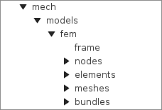
An ArtiSynth FEM model can be rendered in a wide variety of ways, by adjusting the rendering of its nodes, elements, meshes (including the surface and other embedded meshes), and, for FemMuscleModel, muscle bundles. Properties for controlling the rendering include both the standard RenderProps (Section 4.3) as well as more specific properties. These can be set either in code, as described below, or by selecting the desired components (or their lists) and then choosing either Edit render props ... (for standard render properties) or Edit properties ... (for component-specific render properties) from the context menu. As mentioned in Section 4.3, standard render properties are inherited, and so if not explicitly specified within a given component, will assume whatever value has been set in the nearest ancestor component, or their default value. Some component-specific render properties are inherited as well.
One very direct way to control the rendering is to control the visibility of the various component lists. This can be done by selecting them in the navigation panel (Figure 6.18) and then choosing “Set invisible” or “Set visible”, as appropriate. It can also be done in code, as shown in the fragment below making the elements and nodes of an FEM model invisible:
6.12.1 Nodes
Node rendering is controlled by the point render properties of the standard RenderProps. By default, nodes are set to render as gray points one pixel wide, and so are not highly visible. To increase their visibility, and make them easier to select in the viewer, one can make them appear as spheres of a specified radius and color. In code, this can be done using the RenderProps.setSphericalPoints() method, as in this example,
which sets the default rendering for all points within the FEM model (which includes the nodes) to be green spheres of radius 0.01. To restrict this to the node list specifically, one could supply fem.getNodes() instead of fem to setSphericalPoints().
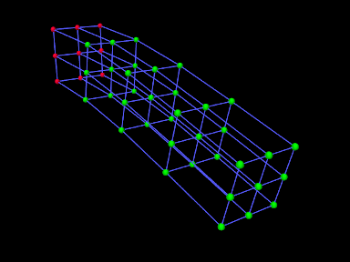
It is also possible to set render properties for individual nodes. For instance, one may wish to mark nodes that are non-dynamic using a different color:
Figure 6.19 shows an FEM model with nodes rendered as spheres, with the dynamic nodes colored green and the non-dynamic ones red.
6.12.2 Elements
By default, elements are rendered as wireframe outlines, using the lineColor and lineWidth properties of the standard render properties, with defaults of “gray” and 1. To improve visibility, one may wish the change the line color or size, as illustrated by the following fragment:
This will set the default line color and width for all components within the FEM model. To restrict this to the elements only, one can specify fem.getElements() (and/or fem.getShellElements()) to the set methods. The fragment above is illustrated in Figure 6.20 (left) for a model created with a call to FemFactory.createHexTorus().
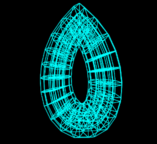
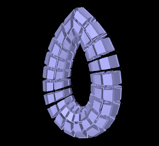
|
Elements can also be rendered as widgets that depict an approximation
of their shape displayed at some fraction of the element’s size (this
shape will be 3D for volumetric elements and 2D for shell
elements). This is controlled using the FemModel3d property elementWidgetSize, which is restricted to the range ![]() and
describes the size of the widgets relative to the element size. If
elementWidgetSize is 0 then no widgets are displayed. The
widget color is controlled using the faceColor and alpha
properties of the standard render properties. The following code
fragment enables element widget rendering for an FEM model, as
illustrated in Figure 6.20 (right):
and
describes the size of the widgets relative to the element size. If
elementWidgetSize is 0 then no widgets are displayed. The
widget color is controlled using the faceColor and alpha
properties of the standard render properties. The following code
fragment enables element widget rendering for an FEM model, as
illustrated in Figure 6.20 (right):
Since setting faceColor for the whole FEM model will also set the default face color for its meshes, one may wish to restrict setting this to the elements only, by specifying fem.getElements() and/or fem.getShellElements() to setFaceColor().
Element widgets can provide a easy way to select specific elements. The elementWidgetSize property is also present as an inherited property in the volumetric and shell element lists (elements and shellElements), as well as individual elements, and so widget rendering can be controlled on a per-element basis.
6.12.3 Surface and other meshes
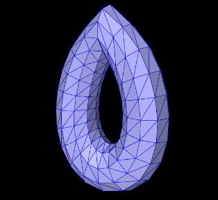
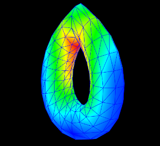
|
A FEM model can also be rendered using its surface mesh and/or other mesh geometry (Section 6.20). How meshes are rendered is controlled by the property surfaceRendering, which can be assigned any of the values shown in Table 6.5. The value None causes nothing to be rendered, while Shaded causes a mesh to be rendered using the standard rendering properties appropriate to that mesh. For polygonal meshes (which include the surface mesh), this will be done according to the face rendering properties in same way as for rigid bodies (Section 3.2.8). These properties include faceColor, shading, alpha, faceStyle, drawEdges, edgeWidth, and edgeColor (or lineColor if the former is not set). The following code fragment sets an FEM surface to be rendered with blue-gray faces and dark blue edges (Figure 6.21, left):
| Value | Description |
|---|---|
| None | mesh is not rendered |
| Shaded | rendered as a mesh using the standard rendering properties |
| Stress | color map of the von Mises stress |
| Strain | color map of the von Mises strain |
| MAPStress | color map of the maximum absolute value principal stress |
| MAPStrain | color map of the maximum absolute value principal strain |
| MaxShearStress | color map of the maximum shear stress |
| MaxShearStrain | color map of the maximum shear strain |
| EnergyDensity | color map of the strain energy density |
Other values of surfaceRendering cause polygonal meshes to be displayed as a color map showing the various stress or strain measures shown in Table 6.5 and described in greater detail in Section 6.11.2. The fragment below sets an FEM surface to be rendered to show the von Mises stress (Figure 6.21, right), while also rendering the edges as dark blue:
The color maps used in stress/strain rendering are controlled using the following additional properties:
- stressPlotRange
-
The range of numeric values associated with the color map. These are either fixed or updated automatically, according to the property stressPlotRanging. Values outside the range are truncated.
- stressPlotRanging
-
Describes if and how stressPlotRange is updated:
- Fixed
-
Range does not change and should be set by the application.
- Auto
-
Range automatically expands to contain the most recently computed values. Note that this does not cause the range to contract.
- colorMap
-
Value is a delegate object that converts stress and strain values to colors. Various types of maps exist, including HueColorMap (the default), GreyscaleColorMap, RainbowColorMap, and JetColorMap. These all implement the ColorMap interface.
All of these properties are inherited and exported both by FemModel3d and the individual mesh components (which are instances of FemMeshComp), allowing mesh rendering to be controlled on a per-mesh basis.
6.12.4 FEM-based muscles
FemMuscleModel and its subcomponents MuscleBundle export additional properties to control the rendering of muscle bundles and their associated fibre directions. These include:
- directionRenderLen
-
A scalar in the range
![[0,1]](mi/mi2248.png) , which if causes the fibre
directions to be rendered within the elements associated with a MuscleBundle (Section 6.9.3). The directions
are rendered as line segments, controlled by the standard line
render properties lineColor and lineWidth, and the value
of directionRenderLen specifies the length of this segment
relative to the size of the element.
, which if causes the fibre
directions to be rendered within the elements associated with a MuscleBundle (Section 6.9.3). The directions
are rendered as line segments, controlled by the standard line
render properties lineColor and lineWidth, and the value
of directionRenderLen specifies the length of this segment
relative to the size of the element. - directionRenderType
-
If directionRenderLen
, this property specifics where the fibre directions should be rendered within muscle bundle
elements. The value ELEMENT causes a single direction to be
rendered at the element center, while INTEGRATION_POINT causes
directions to be rendered at each of the element’s integration points. - elementWidgetSize
-
A scalar in the range
, which if causes the elements
within a muscle bundle to be rendered using an element widget (Section
6.12.2).
Since these properties are inherited and exported by both FemMuscleModel and MuscleBundle, they can be set for the FEM muscle model as a whole or for individual muscle bundles.
The code fragment below sets the element fibre directions for two muscle bundles to be drawn, one in red and one in green, using a directionRenderLen of 0.5. Each bundle runs horizontally along an FEM beam, one at the top and the other at the bottom (Figure 6.22, left):
By default, directionRenderType is set to ELEMENT and so directions are drawn at the element centers. Setting directionRenderType to INTEGRATION_POINT causes the directions to be drawn at each integration point (Figure 6.22, right), which is useful when directions are specified at integration points (Section 6.9.3).
If we are only interested in seeing the elements associated with a muscle bundle, we can use its elementWidgetSize property to draw the elements as widgets (Figure 6.23, left). For this, the last two lines of the fragment above could be replaced with
Finally, if the muscle bundle contains point-to-point fibres (Section 6.9.2), these can be rendered by setting the line properties of the standard render properties. For example, the fibre rendering of Figure 6.23 (right) can be set up using the code
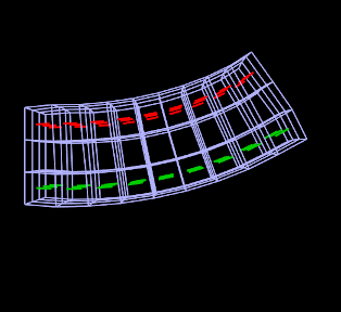

|
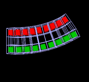

|
6.12.5 Color bars
To display values corresponding to colors, a ColorBar needs to be added to the RootModel. Color bars are general Renderable objects that are only used for visualizations. They are added to the display using the
method in RootModel. Color bars also have a ColorMap associated with it. The following functions are useful for controlling its visualization:
The normalized location specifies sizes relative to the screen size (1 = screen width/height). The location override, if values are non-zero, will override the normalized location, specifying values in absolute pixels. Negative values for position correspond to distances from the left/top. For instance,
will create a bar that is 10% up from the bottom of the screen, 40 pixels from the right edge, with a height occupying 80% of the screen, and width 20 pixels.
Note that the color bar is not associated with any mesh or finite element model. Any synchronization of colors and labels must be done manually by the developer. It is recommended to do this in the RootModel’s prerender(...) method, so that colors are updated every time the model’s rendering configuration changes.
6.12.6 Example: stress/strain plotting with color bars
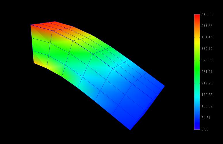
The following model extends FemBeam to render stress, with an added color bar. The loaded model is shown in Figure 6.24.
6.12.7 Cut planes
In addition to stress/strain visualization on its meshes, FEM models can be supplied with one or more cut planes that allow stress or strain values to be visualized on the cross section of the model with the plane.
Cut plane components are implemented by FemCutPlane and can be created with the following constructors:
| FemCutPlane() |
Creates a cut plane aligned with the world origin. |
| FemCutPlane (double res) |
Creates an origin-aligned cut plane with grid resolution res. |
| FemCutPlane (RigidTransform3d TPW) |
Creates a cut plane with pose TPW. |
| FemCutPlane (double res, RigidTransform3d TPW) |
Creates a cut plane with pose TPW and grid resolution res. |
The pose and resolution are described further below. Once created, a cut plane can be added to an FEM model using its addCutPlane() method:
The FEM model methods for handling cut planes include:
| void addCutPlane(FemCutPlane cp) |
Adds a cut plane to the model. |
| int numCutPlanes() |
Queries number of cut planes in the model. |
| FemCutPlane getCutPlanes(int idx) |
Gets the idx-th cut plane in the model. |
| boolean removeCutPlane(FemCutPlane cp) |
Removes a cut plane from the model. |
| void clearCutPlanes() |
Removes all cut planes from the model. |
As with rigid and mesh bodies, the pose of the cut plane gives
its position and orientation relative to world coordinates and is
described by a RigidTransform3d. The
plane itself is aligned with the ![]() -
-![]() plane of this local coordinate
system. More specifically, if the pose is given by
plane of this local coordinate
system. More specifically, if the pose is given by ![]() such that
such that
| (6.38) |
then the plane passes through point ![]() and its normal is given
by the
and its normal is given
by the ![]() axis (third column) of
axis (third column) of ![]() . When rendered in the
viewer, FEM model stress/strain values are displayed as a color map
within the polygonal region formed by the intersection between the
plane and the model’s surface mesh.
. When rendered in the
viewer, FEM model stress/strain values are displayed as a color map
within the polygonal region formed by the intersection between the
plane and the model’s surface mesh.
The following properties of FemCutPlane are used to control how it is rendered in the viewer:
- squareSize
-
A double value, which if
specifies the size of a square that
shows the position of the plane. - resolution
-
A double value, which if
specifies an explicit size (in units
of distance) for the grid cells created within the FEM surface/plane
intersection to interpolate stress/strain values. Smaller values will
give more accurate results but may slow down the rendering
time. Accuracy will also not be improved if the resolution is
significantly less that the size of the FEM elements. If resolution , the grid size is determined automatically based
on the element sizes. - axisLength, axisDrawStyle
-
Identical in function to the axisLength and axisDrawStyle properties for rigid bodies (Section 3.2.8). Specifies the length and style for rendering the local coordinate frame of the cut plane.
- surfaceRendering
-
Describes what is rendered on the surface/plane intersection polygon, according to table 6.5.
- stressPlotRange, stressPlotRanging, colorMap
-
Identical in function to the stressPlotRange, stressPlotRanging and colorMap properties exported by FemModel3d and FemMeshComp (Section 6.12.3). Controls the range and color map associated with the surface rendering.
As with all properties, the values of the above can be accessed either in code using set/get accessors named after the property (e.g., setSurfaceRendering(), getSurfaceRendering()), or within the GUI by selecting the cut plane and then choosing Edit properties ... from the context menu.
6.12.8 Example: FEM model with a cut plane
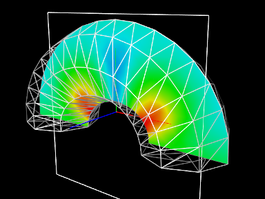
Cut planes are illustrated by the application model defined in
artisynth.demos.tutorial.FemCutPlaneDemo
which creates a simple FEM model in the shape of a half-torus, and then adds a cut plane to render its internal stresses. Its build() method is given below:
After a MechModel is created (lines 27-29), an FEM model
consisting of a half-torus is created, with the bottom nodes set
non-dynamic to provide support (lines 31-43). A cut plane is then
created with a pose that centers it on the world origin and aligns it
with the world ![]() -
-![]() plane (lines 47-49). Surface rendering is set
to Stress, with a fixed color plot range of
plane (lines 47-49). Surface rendering is set
to Stress, with a fixed color plot range of ![]() (lines
52-54). A control panel is created to expose various properties of the
plane (lines 57-63), and then other rendering properties are set: the
default FEM line color is made white (line 67); to avoid visual
clutter FEM elements are made invisible and instead the FEM is
rendered using a wireframe representation of its surface mesh (lines
69-74); and in addition to its render surface, the cut plane is also
displayed using its coordinate axes (with length 0.08) and a square of
size 0.12 (lines 76-78).
(lines
52-54). A control panel is created to expose various properties of the
plane (lines 57-63), and then other rendering properties are set: the
default FEM line color is made white (line 67); to avoid visual
clutter FEM elements are made invisible and instead the FEM is
rendered using a wireframe representation of its surface mesh (lines
69-74); and in addition to its render surface, the cut plane is also
displayed using its coordinate axes (with length 0.08) and a square of
size 0.12 (lines 76-78).
To run this example in ArtiSynth, select All demos > tutorial > FemCutPlaneDemo from the Models menu. When loaded and run, the model should appear as in Figure 6.25. The plane can be repositioned by selecting it in the viewer (by clicking on its square, coordinate axes, or render surface) and then using one of the transformer tools to change its position and/or orientation (see the section “Transformer Tools” in the ArtiSynth User Interface Guide).
Chapter 7 Fields
In modeling applications, particularly those employing FEM methods, situations often arise where it is necessary to describe numeric quantities that vary over some spatial domain. For example, the stiffness parameters of an FEM material may vary at different points within the volumetric mesh. When modeling muscles, the activation direction vector will also typically vary over the mesh.
ArtiSynth provides field components which can be used to represent such spatially varying quantities, together with mechanisms to attach these to certain properties within various materials. Field components can implement either scalar or vector fields. Scalar field components implement the interface ScalarFieldComponent and supply the method
while vector fields implement VectorFieldComponent and supply the method
where T parameterizes a class implementing maspack.matrix.VectorObject. In both cases, the idea is to provide values at arbitrary points over some spatial domain.
For vector fields, the VectorObject represented by T can generally be any fixed-size vector or matrix located in the package maspack.matrix, such as Vector2d, Vector3d, or Matrix3d. T can also be one of the variable-sized objects VectorNd or MatrixNd, although this requires using special wrapper classes and the sizing must remain constant within the field (Section 7.4).
Both ScalarFieldComponent and VectorFieldComponent are subclassed from FieldComponent. The reason for separating scalar and vector fields is simply efficiency: having scalar fields work with the primitive type double, instead of the object Double, requires considerably less storage and somewhat less computational effort.
A field is typically implemented by specifying a finite set of values at discrete locations on an underlying spatial grid and then using an interpolation method to determine values at arbitrary points. The field components themselves are defined within the package artisynth.core.fields.
At present, three types of fields are implemented:
- Grid fields
-
The most basic type of field, in which the values are specified at the vertices of a regular Cartesian grid and then interpolated between vertices. As discussed further in Section 7.1, there are two main types of grid field component: ScalarGridField and VectorGridField<T>.
- FEM fields
-
Fields for which values are specified at the features of an FEM mesh (e.g., nodes, elements or element integration points). As discussed further in Section 7.2, there are six primary types of FEM field component: ScalarNodalField and VectorNodalField<T> (nodes), ScalarElementField and VectorElementField<T> (elements), and ScalarSubElemField and VectorSubElemField<T> (integration points).
- Mesh fields
-
Fields in which values are specified for either the vertices or faces of a triangular mesh. As discussed further in Section 7.3, there are four primary types of mesh field component: ScalarVertexField and VectorVertexField<T> (vertices), and ScalarFaceField and VectorFaceField<T> (faces).
Within an application model, field deployment typically involves the following steps:
-
1.
Create the field component and add it to the model. Grid and mesh fields are usually added to the fields component list of a MechModel, while FEM fields are added to the fields list of the FemModel3d for which the field is defined.
-
2.
Specify field values for the appropriate features (e.g., grid vertices, FEM nodes, mesh faces).
-
3.
If necessary, bind any needed material properties to the field, as discussed further in Section 7.5.
As a simple example of the first two steps, the following code fragment constructs a scalar nodal field associated with an FEM model named fem:
More details on specific field components are given in the sections below.
7.1 Grid fields
A grid field specifies scalar or vector values at the vertices of a regular Cartesian grid and interpolates values between vertices. ArtiSynth currently provides two grid field components in artisynth.core.fields:
where T is any class implementing
maspack.matrix.VectorObject. For both grid types, the
value returned by getValue(p) is determined by finding the grid
cell containing ![]() and then using trilinear interpolation of the
surrounding nodal values. If
and then using trilinear interpolation of the
surrounding nodal values. If ![]() lies outside the grid volume,
then getValue(p) either returns the value at the nearest grid
point
lies outside the grid volume,
then getValue(p) either returns the value at the nearest grid
point ![]() (if the component property clipToGrid is set to true), or else returns a special value indicating that
(if the component property clipToGrid is set to true), or else returns a special value indicating that ![]() is
outside the grid. This special value is ScalarGridField.OUTSIDE_GRID for scalar fields or null for
vector fields.
is
outside the grid. This special value is ScalarGridField.OUTSIDE_GRID for scalar fields or null for
vector fields.
Grid field components are implemented as wrappers around the more basic objects ScalarGrid and VectorGrid<T> defined in maspack.geometry. Applications first create one of these primary grid objects and then use it to create the field component. Instances of ScalarGrid and VectorGrid<T> can be created with constructors such as
where widths gives the grid widths along each of the ![]() ,
, ![]() and
and ![]() axes, res gives the number of cells along each axis, and
for vector grids type is the class type of the
maspack.matrix.VectorObject object parameterized by T. TCL is an optional argument which, if not null,
describes the position and orientation of the grid center with respect
to local coordinates; otherwise, in local coordinates the grid is
centered at the origin and aligned with the
axes, res gives the number of cells along each axis, and
for vector grids type is the class type of the
maspack.matrix.VectorObject object parameterized by T. TCL is an optional argument which, if not null,
describes the position and orientation of the grid center with respect
to local coordinates; otherwise, in local coordinates the grid is
centered at the origin and aligned with the ![]() ,
, ![]() and
and ![]() axes.
axes.
For the vector grid constructors above, T should be a fixed-size vector or matrix, such as Vector3d or Matrix3d. The variable sized objects VectorNd and MatrixNd can also be used with the aid of special wrapper classes, as described in Section 7.4.
By default, grids are axis-aligned and centered at the origin of the world coordinate system. A transform TLW can be specified to place the grid at a different position and/or orientation. TLW represents the transform from local to world coordinates and can be controlled with the methods
If not specified, TLW is the identity and local and world coordinates are the same.
Once a grid is created, it can be used to instantiate a grid field component using one of the constructors
where grid is the primary grid and name is an optional component name. Note that the primary grid is not copied, so any subsequent changes to it will be reflected in the enclosing field component.
Once the grid field component is created, its values can be set by specifying the values at its vertices. The methods to query and set vertex values for scalar and vector fields are
where xi, yj, and zk are the vertex’s indices along the x, y, and z axes, and vi is a general index that should be in the range 0 to field.numVertices()-1 and is related to xi, yj, and zk by
vi = xi + nx*yj + (nx*ny)*zk,
where nx and ny are the number of vertices along the ![]() and
and ![]() axes.
axes.
When computing a grid value using getValue(p), the point p is assumed to be in either grid local or world coordinates, depending on whether the field component’s property localValuesForField is true or false (local and world coordinates are the same unless the primary grid’s local-to-world transform TLW has been set as described above).
To find the spatial position of a vertex within a grid field component, one may use the methods
which return the vertex position in either local or world coordinates depending on the setting of localValuesForField.
The following code example shows the creation of a ScalarGridField, with widths ![]() and a cell
resolution of
and a cell
resolution of ![]() , centered at the origin and
whose vertex values are set to their distance from the origin,
in order to create a simple distance field:
, centered at the origin and
whose vertex values are set to their distance from the origin,
in order to create a simple distance field:
As shown in the example and as mentioned earlier, grid field are generally added to the fields list of a MechModel.
7.2 FEM fields
A FEM field specifies scalar or vector values for the features of an FEM mesh. These can be either the nodes (nodal fields), elements (element fields), or element integration points (sub-element fields). As such, FEM fields provide a way to augment the mesh to store application-specific quantities, and are typically used to bind properties of FEM materials that need to vary over the domain (Section 7.5).
To evaluate getValue(p) at an arbitrary point ![]() , the field
finds the FEM element containing
, the field
finds the FEM element containing ![]() (or nearest to
(or nearest to ![]() , if
, if ![]() is
outside the FEM mesh), and either interpolates the value from the
surrounding nodes (nodal fields), uses the element value directly
(element fields), or interpolates from the integration point values
(sub-element fields).
is
outside the FEM mesh), and either interpolates the value from the
surrounding nodes (nodal fields), uses the element value directly
(element fields), or interpolates from the integration point values
(sub-element fields).
When finding a FEM field value at a point
, getValue(p) is evaluated with respect to the FEM model’s current spatial position, as opposed to its rest position.
FEM fields maintain a default value which describes the value at features for which values are not explicitly set. If unspecified, the default value itself is zero.
In the remainder of this section, it is assumed that vector fields are constructed using fixed-size vectors or matrices, such as Vector3d or Matrix3d. However, it is also possible to construct fields using VectorNd or MatrixNd, with the aid of special wrapper classes, as described in Section 7.4. That section also details a convenience wrapper class for Vector3d.
The three field types are now described in detail.
7.2.1 Nodal fields
Implemented by ScalarNodalField, VectorNodalField<T>, or subclasses of the latter, nodal fields specify their values at the nodes of an FEM mesh. They can be created with constructors such as
where fem is the associated FEM model, defaultValue is the default value, and name is a component name. For vector fields, the maspack.matrix.VectorObject type is parameterized by T, and type gives its actual class type (e.g., Vector3d.class).
Once the field has been created, values can be queried and set at the nodes using methods such as
Here nodeNum refers to an FEM node’s number (which can be obtained using node.getNumber()). Numbers are used instead of indices to identify FEM nodes and elements because they are guaranteed to be persistent in case of mesh editing, and will remain unchanged as long as the node or element is not removed from the FEM model. Note that values don’t need to be set at all nodes, and set values can be unset using the clear methods. For nodes with no value set, the getValue() methods will return the default value.
As a simple example, the following code fragment constructs a ScalarNodalField for an FEM model fem that describes stiffness values at every node of an FEM:
As noted earlier, FEM fields should be stored in the fields list of the associated FEM model.
Another example shows the creation of a field of 3D direction vectors:
When creating a vector field, the constructor needs the class type of the field’s VectorObject. However, for the special case of Vector3d, one may also use the convenience wrapper class Vector3dNodalField, described in Section 7.4.
7.2.2 Element fields
Implemented by
ScalarElementField,
VectorElementField<T>,
or subclasses of the latter, element fields specify their values at
the elements of an FEM mesh, and these values are assumed to be constant within the element. To evaluate getValue(p), the field
finds the containing (or nearest) element for ![]() , and then returns
the value for that element.
, and then returns
the value for that element.
Because values are assumed to be constant within each element, element fields are inherently discontinuous across element boundaries.
The constructors for element fields are analogous to those for nodal fields:
and the methods for setting values at elements are similar as well:
The elements associated with an element field can be either volume or shell elements, which are stored in the FEM component lists elements and shellElements, respectively. Since volume and shell elements may share element numbers, the separate methods getElementValue() and getShellElementValue() are used to access values by element number.
The following code fragment constructs a VectorElementField based on Vector2d that stores a 2D coordinate value at all regular and shell elements:
7.2.3 Sub-element fields
Implemented by ScalarSubElemField, VectorSubElemField<T>, or subclasses of the latter, sub-element fields specify their values at the integration points within each element of an FEM mesh. These fields are used when we need precisely computed information at each of the element’s integration points, and we can’t assume that nodal interpolation will give an accurate enough approximation.
To evaluate getValue(p), the field finds the containing (or
nearest) element for ![]() , extrapolating the integration point values
back to the nodes, and then using nodal interpolation.
, extrapolating the integration point values
back to the nodes, and then using nodal interpolation.
Constructors are similar to those for element fields:
Value accessors are also similar, except that an additional argument k is required to specify the index of the integration point:
The integration point index k should be in the range 0 to ![]() ,
where
,
where ![]() is the total number of integration points for the element in
question and can be queried by the method
numAllIntegrationPoints().
is the total number of integration points for the element in
question and can be queried by the method
numAllIntegrationPoints().
The total number of integration points
, and is used for corotated linear materials. If a SubElemField is being using to supply mesh-varying values to one of the linear material parameters (Section 7.5), then it is important to supply values at the warping point.
The example below shows the construction of a ScalarSubElemField:
First, the field is instantiated with the name "modulus". The code then iterates first through the FEM elements, and then through each element’s integration points, computing values appropriate to each one. A list of each element’s integration points is returned by e.getAllIntegrationPoints(). Having access to the actual integration points is useful in case information about them is needed to compute the field values. In particular, if it is necessary to obtain an integration point’s rest or current (spatial) position, these can be queried as follows:
The regular integration points, excluding the warping point, can be queried using getIntegrationPoints() and numIntegrationPoints() instead of getAllIntegrationPoints() and numAllIntegrationPoints().
7.3 Mesh fields
A mesh field specifies scalar or vector values for the features of a triangular mesh. These can be either the vertices (vertex fields) or faces (face fields). Mesh fields have been introduced in particular to allow properties of contact force behaviors (Section 8.7.2), such as LinearElasticContact, to vary over the contact mesh. Mesh fields can currently be defined only for triangular polygonal meshes.
To evaluate getValue(p) at an arbitrary point ![]() , the field
finds the mesh face nearest to
, the field
finds the mesh face nearest to ![]() , and then either interpolates the
value from the surrounding vertices (vertex fields) or uses the face
value directly (face fields).
, and then either interpolates the
value from the surrounding vertices (vertex fields) or uses the face
value directly (face fields).
Mesh fields make use of the classes PolygonalMesh, Vertex3d, and Face, defined in the package maspack.geometry. They maintain a default value which describes the value at features for which values are not explicitly set. If unspecified, the default value itself is zero.
In the remainder of this section, it is assumed that vector fields are constructed using fixed-size vectors or matrices, such as Vector3d or Matrix3d. However, it is also possible to construct fields using VectorNd or MatrixNd, with the aid of special wrapper classes, as described in Section 7.4. That section also details a convenience wrapper class for Vector3d.
The two field types are now described in detail.
7.3.1 Vertex fields
Implemented by ScalarVertexField, VectorVertexField<T>, or subclasses of the latter, vertex fields specify their values at the vertices of a mesh. They can be created with constructors such as
where mcomp is a mesh component containing the mesh, defaultValue is the default value, and name is a component name. For vector fields, the maspack.matrix.VectorObject type is parameterized by T, and type gives its actual class type (e.g., Vector3d.class).
Once the field has been created, values can be queried and set at the vertices using methods such as
| Scalar fields: | |
|---|---|
| void setValue(Vertex3d vtx, double value) |
Set value for vertex vtx. |
| double getValue(Vertex3d vtx) |
Get value for vertex vtx. |
| double getValue(int vidx) |
Get value for vertex at index vidx. |
| Vector fields with parameterized type T: | |
| void setValue(Vertex3d vtx, T value) |
Set value for vertex vtx. |
| T getValue(Vertex3d vtx) |
Get value for vertex vtx. |
| T getValue(int vidx) |
Get value for vertex at index vidx. |
| All fields: | |
| boolean isValueSet(Vertex3d vtx) |
Query if value set for vertex vtx. |
| void clearValue(Vertex3d vtx) |
Unset value for vertex vtx. |
| void clearAllValues() |
Unset values for all vertices. |
Note that values don’t need to be set at all vertices, and set values can be unset using the clear methods. For vertices with no value set, getValue() will return the default value.
As a simple example, the following code fragment constructs a ScalarVertexField for a mesh contained in the MeshComponent mcomp that describes contact stiffness values at every vertex:
As noted earlier, mesh fields are usually stored in the fields list of a MechModel.
Another example shows the creation of a field of 3D direction vectors:
When creating a vector field, the constructor needs the class type of the field’s VectorObject. However, for the special case of Vector3d, one may also use the convenience wrapper class Vector3dVertexField, described in Section 7.4.
7.3.2 Face fields
Implemented by
ScalarFaceField,
VectorFaceField<T>,
or subclasses of the latter, face fields specify their values at the
faces of a polygonal mesh, and these values are assumed to be constant within the face. To evaluate getValue(p), the field
finds the containing (or nearest) face for ![]() , and then returns the
value for that face.
, and then returns the
value for that face.
Because values are assumed to be constant within each face, face fields are inherently discontinuous across face boundaries.
The constructors for face fields are analogous to those for vertex fields:
and the methods for setting values at faces are similar as well, where fidx refers to the face index:
The following code fragment constructs a VectorFaceField based on Vector2d that stores a 2D coordinate value at all faces of a mesh:
7.4 Fields for VectorNd, MatrixNd and Vector3d
The vector fields described above can be implemented for most fixed-size vectors and matrices defined in the package maspack.matrix (e.g., Vector2d, Vector3d, Matrix3d). However, if vectors or matrices with different size are needed, it is also possible to create vector fields using VectorNd and MatrixNd, provided that the sizing remain constant within any given field. This is achieved using special wrapper classes that contain the sizing information, which is supplied in the constructors. For convenience, wrapper classes are also provided for vector fields that use Vector3d, since that vector size is quite common.
For vector FEM and mesh fields, the complete set of wrapper classes is listed below:
| Class | base class | vector type T |
|---|---|---|
| Vector FEM fields: | ||
| Vector3dNodalField | VectorNodalField<T> | Vector3d |
| VectorNdNodalField | VectorNodalField<T> | VectorNd |
| MatrixNdNodalField | VectorNodalField<T> | MatrixNd |
| Vector3dElementField | VectorElementField<T> | Vector3d |
| VectorNdElementField | VectorElementField<T> | VectorNd |
| MatrixNdElementField | VectorElementField<T> | MatrixNd |
| Vector3dSubElemField | VectorSubElemField<T> | Vector3d |
| VectorNdSubElemField | VectorSubElemField<T> | VectorNd |
| MatrixNdSubElemField | VectorSubElemField<T> | MatrixNd |
| Vector mesh fields: | ||
| Vector3dVertexField | VectorVertexField<T> | Vector3d |
| VectorNdVertexField | VectorVertexField<T> | VectorNd |
| MatrixNdVertexField | VectorVertexField<T> | MatrixNd |
| Vector3dFaceField | VectorFaceField<T> | Vector3d |
| VectorNdFaceField | VectorFaceField<T> | VectorNd |
| MatrixNdFaceField | VectorFaceField<T> | MatrixNd |
These all behave identically to their base classes, except that their constructors omit the type argument (since this is built into the class definition) and, for VectorNd and MatrixNd, supply information about the vector or matrix sizes. For example, constructors for the FEM nodal fields include
where vecSize, rowSize and colSize give the sizes of the VectorNd or MatrixNd objects within the field. Constructors for other field types are equivalent and are described in their API documentation.
For grid fields, one can use either VectorNdGrid or MatrixNdGrid, both defined in maspack.geometry, as the primary grid used to construct the field. Constructors for these include
7.5 Binding material properties
A principal purpose of field components is to enable certain FEM material properties to vary spatially over the FEM geometry. Many material properties can be bound to a field, so that when they are queried internally by the solver at the integration points for each FEM element, the field value at that integration point is used instead of the regular property value. Likewise, some properties of contact force behaviors, such as the YoungsModulus and thickness properties of LinearElasticContact (Section 8.7.3) can be bound to a field that varies over the contact mesh geometry.
To bind a property to a field, it is necessary that
-
1.
The type of the field matches the value of the property;
-
2.
The property is itself bindable.
If the property has a double value, then it can be bound to any ScalarFieldComponent. Otherwise, if the property has a value T, where T is an instance of maspack.matrix.VectorObject, then it can be bound to a vector field.
Bindable properties export two methods with the signature
where XXX is the property name and F is an appropriate field type.
As long as a property XXX is bound to a field, its regular value will still appear (and can be set) through widgets in control or property panels, or via its getXXX() and setXXX() accessors. However, the regular value won’t be used internally by the FEM simulation.
For example, consider the YoungsModulus property, which is present in several FEM materials, including LinearMaterial and NeoHookeanMaterial. This has a double value, and is bindable, and so can be bound to a ScalarFieldComponent as follows:
It is important to perform field bindings on materials before they are set in an FEM model (or one of its subcomponents, such as MuscleBundles). That’s because the setMaterial() method copies the input material, and so any settings made on it afterwards won’t be seen by the FEM:
// works: field will be seen by the copied version of ’mat’ mat.setYoungsModulusField (field); fem.setMaterial (mat); // does NOT work: field not seen by the copied version of ’mat’ fem.setMaterial (mat); mat.setYoungsModulusField (field);
To unbind YoungsModulus, one can call
Usually, FEM fields are used to bind properties in FEM materials while mesh fields are used for contact properties, but other fields can be used, particularly grid fields. To understand this a bit better, we discuss briefly some of the internals of how binding works. When evaluating stresses, FEM materials have access to a FemFieldPoint object that provides information about the integration point, including its element, nodal weights, and integration point index. This can be used to rapidly evaluate values within nodal, element and sub-element FEM fields. Likewise, when evaluating contact forces, contact materials like LinearElasticContact have access to a MeshFieldPoint object that describes the contact point position as a weighted sum of mesh vertex positions, which can then be used to rapidly evaluate values within vertex or face mesh fields. However, all fields, regardless of type, implement methods for determining values at both FemFieldPoints and MeshFieldPoints:
If necessary, these methods simply fall back on the getValue(Point3d) method, which is defined for all fields and works relatively fast for grid fields.
There are some additional details to consider when binding FEM material properties:
-
1.
When binding to a grid field, one has the choice of whether to use the grid to represent values with respect to the FEM’s rest position or spatial position. This can be controlled by setting the useFemRestPositions property of the grid field, the default value for which is true.
-
2.
When binding the bulkModulus property of an incompressible material, it is best to use a nodal field if the FEM model is using nodal-based soft incompressibility (i.e., the model’s softIncompMethod property is set to either NODAL or AUTO; Section 6.7.3). That’s because soft nodal incompressibility requires evaluating the bulk modulus property at nodes instead of integration points, which is much easier to do with a nodal-based field.
7.5.1 Example: FEM with variable stiffness
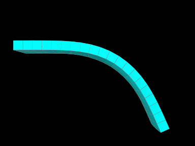
A simple model demonstrating a stiffness that varies over an FEM mesh is defined in
artisynth.demos.tutorial.VariableStiffness
It consists of a simple thin hexahedral beam with a linear material
for which the Young’s modulus ![]() is made to vary nonlinearly along the
x axis of the rest position according to the formula
is made to vary nonlinearly along the
x axis of the rest position according to the formula
| (7.0) |
The model’s build method is given below:
Lines 6-10 create the hex FEM model and shift it so that the left side
is aligned with the origin, while lines 12-17 fix the leftmost
nodes. Lines 21-27 create a scalar nodal field for the Young’s modulus,
with lines 23-24 computing ![]() according to (7.0).
The field is then bound to a linear material which is then set in the
model (lines 30-32).
according to (7.0).
The field is then bound to a linear material which is then set in the
model (lines 30-32).
The example can be run in ArtiSynth by selecting All demos > tutorial > VariableStiffness from the Models menu. When run, the beam will bend under gravity, but mostly on the right side, due to the much higher stiffness on the left (Figure 7.1).
7.5.2 Example: specifying FEM muscle directions
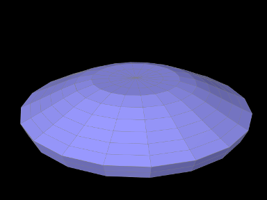 |
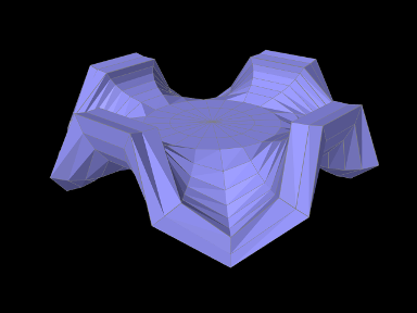 |
Another example involves using a Vector3d field to specify the muscle activation directions over an FEM model and is defined in
artisynth.demos.tutorial.RadialMuscle
When muscles are added using MuscleBundles ( Section 6.9), the muscle directions are stored and handled internally by the muscle bundle itself. However, it is possible to add a MuscleMaterial directly to the elements of an FEM model, using a MaterialBundle (Section 6.8), in which case the directions need to be set explicitly using a field.
The model’s build method is given below:
Lines 5-19 create a thin cylindrical FEM model, centered on the
origin, with radius ![]() and height
and height ![]() , consisting of hexes with
wedges at the center, with two layers of elements along the
, consisting of hexes with
wedges at the center, with two layers of elements along the ![]() axis
(which is parallel to the cylinder axis). Its base material is set to
a neo-hookean material. To keep the model from falling under gravity,
all nodes whose distance to the
axis
(which is parallel to the cylinder axis). Its base material is set to
a neo-hookean material. To keep the model from falling under gravity,
all nodes whose distance to the ![]() axis is less than
axis is less than ![]() are fixed.
are fixed.
Next, a Vector3d field is created to specify the directions, on a
per-element basis, for the muscle material which will be added subsequently
(lines 21-32). While we could create an instance of VectorElementField<Vector3d>, we use
Vector3dElementField, since this
is available and provides additional functionality (such as the
ability to render the directions). Directions are set to lie outward
in a radial direction perpendicular to the ![]() axis, and since the
model is centered on the origin, they can be computed easily by first
computing the element centroids, removing the
axis, and since the
model is centered on the origin, they can be computed easily by first
computing the element centroids, removing the ![]() component, and then
normalizing. In order to give the muscle action an upward bias, we
only set directions for elements in the upper layer. Direction values
for elements in the lower layer will then automatically have a default
value of 0, which will cause the muscle material to not apply any
stress.
component, and then
normalizing. In order to give the muscle action an upward bias, we
only set directions for elements in the upper layer. Direction values
for elements in the lower layer will then automatically have a default
value of 0, which will cause the muscle material to not apply any
stress.
We next add to the model a muscle material whose directions will be determined by the field. To hold the material, we first create and add a MaterialBundle which is set to act on all elements (line 35-36). Then we set this bundle’s material to SimpleForceMuscle, which adds a stress along the muscle direction that equals the excitation value times the value of its maxStress property, and bind the material’s restDir property to the direction field (lines 37-39).
Finally, we create and add a control panel to allow interactive control over the muscle material’s excitation property (lines 42-44), and set some rendering properties for the FEM model.
The example can be run in ArtiSynth by selecting All demos > tutorial > RadialMuscle from the Models menu. When it is first run, it falls around the edges under gravity (Figure 7.2, top). Applying an excitation causes a radial contraction which pulls the edges upward and, if high enough, causes them to buckle (Figure 7.2, bottom).
7.6 Visualizing fields
It is often useful to be able to visualize the contents of a field, particularly for testing and validation purposes. ArtiSynth field components export various properties that allow their values to be visualized in the viewer.
As described in Section 7.6.3, the grid field components, ScalarGridField and VectorGridField, are not visible by default, and so must be made visible to enable visualization.
7.6.1 Scalar fields
Scalar fields are visualized by means of a color map that associates scalar values with colors, with the actually visualization typically taking the form of either a discrete set of colored points, or a colored surface embedded within the field. The color map and its associated visualization is controlled by the following properties:
- colorMap
-
An instance of the ColorMap interface that controls how field values are mapped onto colors. Various types of maps exist, including GreyscaleColorMap, HueColorMap, RainbowColorMap, and JetColorMap, each containing subproperties controlling how its colors are generated.
- renderRange
-
Composite property of the type ScalarRange that controls the range of field values used for color map rendering. Subproperties include interval, which gives the value range itself, and updating, which specifies how this interval is determined from the field: FIXED (interval can be set manually), AUTO_EXPAND (interval is expanded to accommodate all field values), and AUTO_FIT (interval is tightly fit to the field values). Note that for AUTO_EXPAND and AUTO_FIT, the interval is determined by the range of field values, and not the values that actually appear in the visualization. The latter can differ from the former when the surface does not cover the whole field, or lies outside the field, resulting in extrapolated values that fall outside the field’s range. Setting updating to FIXED and manually setting the interval can be useful in such cases.
- visualization
-
An enumerated type that specifies the actual type of rendering used to visualize the field (e.g., points, surface, or other). While its definition is specific to the field type (ScalarFemField.Visualization for FEM fields, ScalarMeshField.Visualization for mesh fields; ScalarGridField.Visualization for grid fields), overall it will have one of five values (POINT, SURFACE, ELEMENT, FACE, or OFF) described further below.
- volumeElemsVisible
-
A boolean property, exported by ScalarElementField and ScalarSubElemField, which if false causes volumetric element values to be ignored in the visualization. The default value is true.
- shellElemsVisible
-
A boolean property, exported by ScalarElementField and ScalarSubElemField, which if false causes shell element values to be ignored in the visualization. The default value is true.
- renderProps
-
Basic rendering properties of the field component that are used to control some aspects of the rendering (Section 4.3), as described below.
The above properties can be accessed either interactively in the GUI, or in code, using the field’s methods getColorMap(), setColorMap(map), getRenderRange(), setRenderRange(range), getVisualization(), and setVisualization(type).
While the enumerated type associated with the visualization property is specific to the field type, all values together will be one of the following:
- POINT
-
Field is visualized using colored points placed at the features used to define the field (e.g., nodes, element centers, or integration points for FEM fields; vertices and face centers for mesh fields; vertices for grid fields). How the points are displayed is controlled using the pointStyle subproperty of the grid’s renderProps, with their size controlled either by pointRadius or pointSize (if the pointStyle is POINT).
- SURFACE
-
Field is visualized using a colored surface, specified by one or more polygonal meshes associated with the field, where the values at mesh vertices are either determined directly, or interpolated from, the field. This type of visualization is available for ScalarNodalField, ScalarSubElemField, ScalarVertexField and ScalarGridField. For ScalarVertexField, the mesh is the mesh associated with the field itself. Otherwise, the meshes are supplied by external mesh components that are attached to the field as render meshes, as described in Section 7.6.4. For ScalarNodalField and ScalarSubElemField, these mesh components must be either FemMeshComps (Section 6.3) or FemCutPlanes (Section 6.12.7) associated with the FEM model, and may include its surface mesh; while for ScalarGridField, the mesh components are fixed mesh bodies (Section 3.3.1).
- ELEMENT
-
Used only by ScalarElementField, allows the field to be visualized by element shaped widgets that are colored according to each element’s field value and the color map. The size of the widget, relative to the true element size, is controlled by the property elementWidgetSize, which is a scalar in the range
. - FACE
-
Used only by ScalarFaceField, allows the field to be visualized by rendering the associated field mesh, with each face colored according to its field value and the color map.
- OFF
-
No visualization (the default value).
7.6.2 Vector fields
Vector fields can be visualized, when possible, by drawing three dimensional line segments, with a length proportional to the field value, originating at the features used to define the field (nodes, element centers, or integration points for FEM fields; vertices and face centers for mesh fields; vertices for grid fields). This can done for any field whose vector type is an instance of Vector (which includes Vector2d, Vector3d, and VectorNd) by mapping the vector values onto a 3-vector. This means ignoring element values for vectors whose size is greater than 3, and setting higher element values to 0 for vectors whose size is less than 3.
Vector field rendering is controlled by the following properties:
- renderScale
-
A double which scales the vector field value to determine the length of the drawn line segment. The default value is 0, implying that no vectors are drawn.
- renderProps
-
Basic rendering properties of the field component, as described in Section 4.3. How the lines are displayed is controlled by the line subproperties, with the color specified by lineColor, the style by lineStyle (LINE, CYLINDER, SOLID_ARROW, SPINDLE), and the size by either lineRadius or lineWidth (if the lineStyle is LINE).
7.6.3 Grid fields
As mentioned above, the grid field components, ScalarGridField and VectorGridField, are not visible by default, and so must be made visible to enable visualization:
By default, grid field components also render their grid edges, using the edge subproperties of renderProps (drawEdges, edgeWidth, and edgeColor). If edgeColor is not set (i.e., is set to null), the lineColor subproperty is used instead. Grid components also have a renderGrid property which can be set to false to disable rendering of the grid.
For VectorGridField, when rendering the grid and visualizing the vectors, one can make them different colors by using the edgeColor subproperty of renderProps to set the grid color:
7.6.4 Render meshes
The scalar fields ScalarNodalField, ScalarSubElemField, and ScalarGridField all make use of render meshes when being visualized using SURFACE visualization. These are a collection of one or more components, each providing a polygonal mesh that defines a surface for rendering a color map of the field, based on values at the mesh vertices that are themselves determined from the field. For ScalarNodalField and ScalarSubElemField), the mesh components must be either FemMeshComps contained within the FEM’s meshes list (Section 6.3) or FemCutPlanes contained within the FEM’s cutPlanes list (Section 6.12.7), while for ScalarGridField, they are FixedMeshBodys (Section 3.3.1) that are usually contained within the MechModel.
Adding render meshes to a field must be done in code. For ScalarNodalField and ScalarSubElemField, the set of rendering meshes is controlled by the following methods:
| void addRenderMeshComp (FemMesh mcomp) |
Add the render mesh component mcomp. |
| boolean removeRenderMeshComp (FemMesh mcomp) |
Remove the render mesh component mcomp. |
| FemMesh getRenderMeshComp (idx) |
Return the idx-th render mesh component. |
| int numRenderMeshComps() |
Return the number of render mesh components. |
| void clearRenderMeshComps() |
Clear all the render mesh components. |
Equivalent methods exist for ScalarGridField, using FixedMeshBody instead of FemMesh.
The following should be noted with respect to render meshes:
-
•
A render mesh can be created for the sole purpose of visualizing a field. A rectangle often does well for this purpose.
-
•
Rendering of the visualization is done by the field component, not the render mesh component(s), and so it is usually necessary to make the latter invisible to avoid rendering conflicts.
-
•
Render meshes should have a large enough number of vertices and triangles to support the resolution required to visualize the field properly.
-
•
One can often use the GUI transformer tools to interactively adjust a render mesh’s pose (see “Transformer tools” in the ArtiSynth User Interface Guide), allowing the user to move a render surface throughout the field. For FixedMeshBody and FemCutPlane, the tools change the component’s pose, while for FemMeshComp, they change the location of its embedding within the FEM.
Transformer tools have no effect on FEM meshes which are auto-generated, such as the default surface mesh.
As a simple example, the following code fragment creates a square render mesh for a ScalarGridField:
7.6.5 Example: Visualizing a scalar nodal field
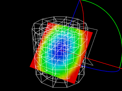
A simple application that uses a FemCutPlane to visualize a ScalarNodalField is defined in
artisynth.demos.tutorial.ScalarFieldVisualization
The build() method for this is shown below:
After first creating a MechModel (lines 2-3), a cylindrical
hexahedral FEM model is created to contain the field, with its top
nodes fixed to allow it to deform under gravity (lines 13-17). A ScalarNodalField is then defined for this FEM, where the value at
each node is set to ![]() , with
, with ![]() being the radial distance from the
node to the FEM’s central axis (lines 21-27).
being the radial distance from the
node to the FEM’s central axis (lines 21-27).
To visualize the field, a FemCutPlane is created with its pose
set to align it with the ![]() -
-![]() plane and then added to the FEM model
(lines 31-33). The field’s visualization is then set to SURFACE
and the cut plane is added to it as a render mesh (lines 36-37). At
lines 40-44, a control panel is created to allow interactive
adjustment of the field’s visualization, renderRange, and
colorMap properties. Finally, render properties are set: the FEM
line color (used to render element edges) is set to blue-gray (line
48); the cut plane’s surface rendering is set to None to avoid
interfering with the field rendering, and axis rendering is enabled to
make the field visible and selectable even if it doesn’t intersect the
FEM (lines 51-53); and, for POINT visualization, the field is
set to render points as spheres with a radius of
plane and then added to the FEM model
(lines 31-33). The field’s visualization is then set to SURFACE
and the cut plane is added to it as a render mesh (lines 36-37). At
lines 40-44, a control panel is created to allow interactive
adjustment of the field’s visualization, renderRange, and
colorMap properties. Finally, render properties are set: the FEM
line color (used to render element edges) is set to blue-gray (line
48); the cut plane’s surface rendering is set to None to avoid
interfering with the field rendering, and axis rendering is enabled to
make the field visible and selectable even if it doesn’t intersect the
FEM (lines 51-53); and, for POINT visualization, the field is
set to render points as spheres with a radius of ![]() (line 55).
(line 55).
To run this example in ArtiSynth, select All demos > tutorial > ScalarFieldVisualization from the Models menu. Users can employ the control panel to adjust the visualization, the render range, and the color map. When SURFACE visualization is selected, the field will be rendered onto the FEM/plane intersection defined by the cut plane. Simulating the model will cause the FEM to deform, deforming this intersection with it. Clicking on the intersection surface or the cut plane axes will cause the cut plane to be selected. Its pose can then be adjusted using the GUI transformer tools (see “Model Manipulation” in the ArtiSynth User Interface Guide), as shown in Figure 7.3.
When the updating property of the render range is set to AUTO_FIT, the range will be automatically set to the range of values in the field, and not the values evaluated over the render surface. The latter may exceed the former due to extrapolation when the surface extends outside of the FEM, in which case the visualization will appear to saturate. While this is not generally a concern because FEM field values are unreliable outside of the FEM, one can override this effect by setting the updating property to FIXED and setting the range interval manually.
7.6.6 Examples: Visualizing other fields
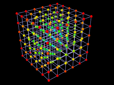
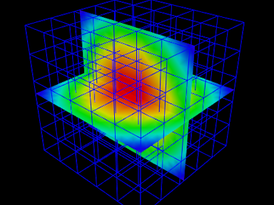
|
Numerous examples exist for creating and visualizing other field types:
artisynth.demos.fem.ScalarNodalFieldDemo artisynth.demos.fem.ScalarElementFieldDemo artisynth.demos.fem.ScalarSubElemFieldDemo artisynth.demos.fem.VertexNodalFieldDemo artisynth.demos.fem.VertexElementFieldDemo artisynth.demos.fem.VertexSubElemFieldDemo artisynth.demos.mech.ScalarVertexFieldDemo artisynth.demos.mech.ScalarFaceFieldDemo artisynth.demos.mech.ScalarGridFieldDemo artisynth.demos.mech.VertexVertexFieldDemo artisynth.demos.mech.VertexFaceFieldDemo artisynth.demos.mech.VertexGridFieldDemo
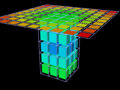
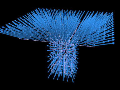
|
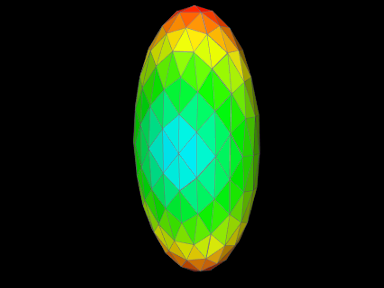
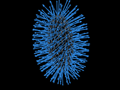
|
Chapter 8 Contact and Collision
ArtiSynth supports contact and collisions between various collidable bodies, including rigid bodies and FEM models, through a collision handling mechanism built into MechModel. Collisions are disabled by default, but can be enabled between specific pairs of bodies, or between general categories of rigid and deformable bodies (Section 8.1). Collisions are supported between any body that implements the interface Collidable.
Collision detection works by finding the intersecting regions between the collision meshes of collidable bodies, and then using the intersection information to determine contact points and their associated constraints (Section 8.4). Collision meshes must be instances of PolygonalMesh and must be triangular; mesh requirements are described in more detail in Section 8.3. Typically, a collision mesh is the same as the body’s surface mesh, but other meshes (or collections of meshes) can be specified instead (Section 8.3).
Detailed aspects of the collision behavior, such as friction, optional compliance and damping terms, methods used to determine contacts, and various tolerances, can be controlled using CollisionBehavior objects (Section 8.2). Collisions can be visualized by rendering contact normals, forces, intersection contours, and contact pressures (Section 8.5), and information about specific collisions, including contact data, forces, and pressures, can also be monitored as the simulation proceeds (Section 8.8).
It is also possible to explicitly control contact forces by making them an explicit function of penetration depth (Section 8.7); in particular, this capability is used to support elastic foundation contact (Section 8.7.3).
It should be understood that collision handling can be computationally
expensive and, due to its discontinuous nature, may be less accurate
than other aspects of the simulation. ArtiSynth therefore provides a
number of ways to selectively control collision handling between
different pairs of bodies. Collision handling is also challenging
because if collisions are enabled among ![]() objects, then one needs to
be able to easily specify the characteristics of up to
objects, then one needs to
be able to easily specify the characteristics of up to ![]() collision interactions, while also managing the fact that these
interactions are highly transient. In ArtiSynth, collision handling
is managed by a
CollisionManager that is a
subcomponent of each
MechModel. The collision
manager maintains default collision behaviors among certain groups of
collidable objects, while also allowing the user to override the
default behaviors by setting specific behaviors for any given pair of
collidables.
collision interactions, while also managing the fact that these
interactions are highly transient. In ArtiSynth, collision handling
is managed by a
CollisionManager that is a
subcomponent of each
MechModel. The collision
manager maintains default collision behaviors among certain groups of
collidable objects, while also allowing the user to override the
default behaviors by setting specific behaviors for any given pair of
collidables.
Within ArtiSynth, the terms collision and contact are used somewhat interchangeably, although we acknowledge that in the literature, collision is generally understood to refer to the transient process that occurs when bodies first come into contact, while contact refers to the more persistent situation as the bodies remain together.
8.1 Enabling collisions
This section describes how to enable collisions in code. However, it is also possible to set some aspects of collision behavior using the ArtiSynth GUI. See the section “Collision handling” in the ArtiSynth User Interface Guide.
ArtiSynth can simulate collisions between bodies that implement the interface Collidable. Collidable bodies are further subdivided into those that are rigid and those that are deformable, according to whether their isDeformable() method returns true. Rigid collidables include RigidBody, while deformable collidables include FEM models (FemModel3d), their mesh components (FemMeshComp), and skinned meshes (SkinMeshBody, Chapter 11). Because of the computational cost, collision detection is turned off by default and must be explicitly enabled when a model is built. Collisions can be enabled between specific pairs of bodies, or between general groupings of rigid and deformable bodies.
Collision handling is implemented by a model’s MechModel, which contains a CollisionManager subcomponent that keeps track of which bodies are colliding and computes the constraints and forces needed to enforce the collision behaviors. The collision manager itself can be accessed by the MechModel method
and can be used to query and set various collision properties, as described further below.
8.1.1 Collisions between specific bodies
As indicated above, collidable bodies are typically components such as rigid bodies or FEM models. Given two collidable bodies collidable0 and collidable1, the simplest way to enable collisions between them is with the MechModel methods
The first method enables collisions without friction, while the second enables collisions with friction as specified by mu, which is the coefficient of Coulomb (or dry) friction. The mu value is ignored if enabled is false. Specifying a mu value of 0 disables friction, and the friction coefficient can also be left undefined by specifying a mu value less than 0, in which case the coefficient is inherited from the global friction value accessed by the MechModel methods
More detailed control over collision behavior can be achieved using the method
where behavior is a CollisionBehavior object (Section8.2.1) that specifies both enabled and mu, along with other, more detailed collision properties (see Section 8.2.1).
The setCollisionBehavior() methods work by adding a CollisionBehavior object to the collision manager as a subcomponent. With the method setCollisionBehavior(collidable0,collidable1,behavior), the behavior object is created and supplied by the application. With the other methods, the behavior object is created automatically and returned by the method. Once a behavior has been specified, it can then be queried using
This method will return null if no behavior for the pair in question has been explicitly set using one of the setCollisionBehavior() methods.
One should normally avoid enabling collisions between bodies that are otherwise connected, for example, adjacent bodies in a linkage connected by joints, in order to avoid conflicts between the connection and the collision behavior. If collision interaction is required between parts of two connected bodies, this can be achieved in various ways as described in Section 8.3.
Because behaviors are proper components, it is not permissible to add them to the collision manager twice. Specifically, the following will produce an error:
CollisionBehavior behav = new CollisionBehavior(); behav.setDrawIntersectionContours (true); mech.setCollisionBehavior (col0, col1, behav); mech.setCollisionBehavior (col2, col3, behav); // ERRORHowever, if desired, a new behavior can be created from an existing one:
CollisionBehavior behav = new CollisionBehavior(); behav.setDrawIntersectionContours (true); mech.setCollisionBehavior (col0, col1, behav); behav = new CollisionBehavior(behav); mech.setCollisionBehavior (col2, col3, behav); // OK
8.1.2 Default collisions between groups
For convenience, it is also possible to specify default collision behaviors between different groups of collidables.
The default collision behavior between all collidables can be controlled using the MechModel methods
where enabled, mu and behavior act as described in Section 8.1.1.
Because of the possible computational expense of collision detection, default collision behaviors should be used with care.
In addition, a default collision behavior can be set for generic groups of collidables using the MechModel methods
where group0 and group1 are static instances of Collidable.Group that represent the groups described in Table 8.1. The groups Collidable.Rigid and Collidable.Deformable denote collidables that are rigid and deformable, respectively. The group Collidable.AllBodies denotes both rigid and deformable bodies, and Collidable.Self is used to enable self-collision, which is described in greater detail in Section 8.3.2.
| Collidable group | description |
|---|---|
| Collidable.Rigid | rigid collidables (e.g., rigid bodies) |
| Collidable.Deformable | deformable collidables (e.g, FEM models) |
| Collidable.AllBodies | rigid and deformable collidables |
| Collidable.Self | enables self-intersection for compound deformable collidables |
| Collidable.All | rigid and deformable collidables and self-intersection |
A call to one of the setDefaultCollisionBehavior() methods will override the effects of previous calls. So for instance, the code sequence
will initially enable collisions between all bodies with a friction coefficient of 0, then disable collisions between deformable and rigid bodies, and finally re-enable collisions between all bodies with a friction coefficient of 0.2.
The default collision behavior between any pair of collidable groups can be queried using
where group0 and group1 are restricted to the primary groups Collidable.Rigid, Collidable.Deformable, and Collidable.Self, since individual behaviors are not maintained for the composite groups Collidable.AllBodies and Collidable.All.
Specific collision behaviors set using the setCollisionBehavior() methods of Section 8.1.1 will override any default collision settings. In addition, the second argument collidable1 of these methods can describe either an individual collidable, or one of the groups of Table 8.1. For example, the code fragment
will enable collisions between bodA and all deformable collidables (with friction 0.1), as well as femB and all deformable and rigid collidables (with friction 0.0), while specifically disabling collisions between bodA and femB.
To determine the actual behavior controlling collisions between two collidables (whether due to a default behavior or one specified using setCollisionBehavior()), one may use the method
where collidable0 and collidable1 must both be specific collidable components and cannot be a group (such as Collidable.Rigid or Collidable.All). If one of the collidables is a compound collidable (Section 8.3.2), or has a collidability setting (Section 8.2.2) that prevents collisions, there may be no consistent acting behavior, in which case the method returns null.
Collision behaviors take priority over each other in the following order:
-
1.
Behaviors specified using setCollisionBehavior() involving two specific collidables.
-
2.
Behaviors specified using setCollisionBehavior() involving one specific collidable and a group of collidables (indicated by a Collidable.Group), with later specifications taking priority over earlier ones.
-
3.
Default behaviors specified using setDefaultCollisionBehavior().
A collision behavior specified with setCollisionBehavior() can later be removed using
and all such behaviors in a MechModel can be removed with
Note that this latter call does not remove default behaviors specified with setDefaultCollisionBehavior().
8.1.3 Example: collision with a plane
A simple model illustrating collision between two jointed rigid bodies and a plane is defined in
artisynth.demos.tutorial.JointedCollide
This model is simply a subclass of RigidBodyJoint that overrides the build() method to add an inclined plane and enable collisions between it and the two connected bodies:
The superclass build() method called at line 3 creates everything contained in RigidBodyJoint. The remaining code then alters that model: bodyB is set to be dynamic (line 5) so that it will fall freely, and an inclined plane is created from a thin box that is translated and rotated and then set to be non-dynamic (lines 8-11). Finally, collisions are enabled by setting the default collision behavior (line 14), and then specifically disabling collisions between bodyA and bodyB (line 15). As indicated above, the latter step is necessary because the joint would otherwise keep the two bodies in a permanent state of collision.
To run this example in ArtiSynth, select All demos > tutorial > JointedCollide from the Models menu. The model should load and initially appear as in Figure 8.1. Running the model (Section 1.5.3) will cause the jointed assembly to collide with and slide off the inclined plane.
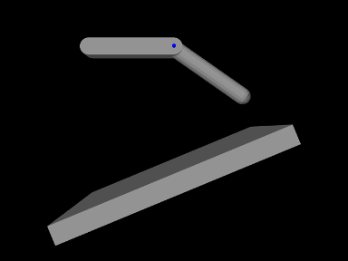
8.1.4 Collisions for FEM models
Both FemModel3d and FemMeshComp implement Collidable. By default, a FemModel3d uses its surface mesh as the collision surface, while FemMeshComp will use the mesh it contains (although collisions will only occur if this is a triangular polygonal mesh).
Because FemModel3d contains other collidables as subcomponents, it is considered a compound collidable, as discussed further in Section 8.3.2. In particular, since FemMeshComp is also a Collidable, we can enable collisions with any embedded mesh inside an FEM. Any forces resulting from the collision are then automatically transferred back to the underlying nodes of the model using Equation (6.4).
Note: Collisions involving shell elements are not yet fully supported. This relates to the fact that shells are thin and can therefore pass through each other easily in a single time step, and also that meshes associated with shell elements are usually not closed. However, collisions should work properly if
- 1.
The collision meshes do not pass completely through each other in a single time step;
- 2.
Collisions do not occur near open mesh edges.
Restriction 2 can often be relaxed if the collider type is set to TRI_INTERSECTION (Section 8.4.2).
8.1.5 Example: FEM models and rigid bodies
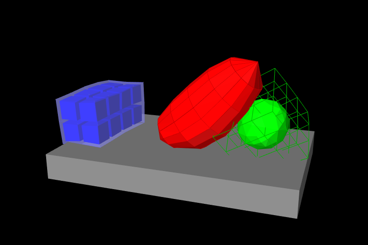
An example of FEM collisions is shown in Figure 8.2. The full source code can be found in the ArtiSynth repository under artisynth.demos.tutorial.FemCollisions. The model contains a rigid body table and three FEM models: a beam (blue), an ellipsoid (red), and a hex block containing an embedded spherical mesh (green). The collision-enabling code is as follows:
This enables collisions between the ellipsoid and the beam, table and embedded sphere, and between the table and the beam and embedded sphere. However, collisions are not enabled between the block itself and any other components; notice in the figure that the block surface passes through the table and ellipsoid.
8.2 Collision behaviors and collidability
8.2.1 Collision behaviors
As mentioned above, CollisionBehavior objects can be used to control other aspects of contact beyond friction and enabling. This may be done by setting the CollisionBehavior properties listed below. Except where otherwise indicated, these properties are also exported by the collision manager, where they can be used to provide global default settings for all collisions.
In addition to these properties, CollisionBehavior and CollisionManager export other properties that can be used to control the rendering of collisions, as described in Section 8.5.
- enabled
-
A boolean that determines if collisions are enabled. Not present in the collision manager.
- friction
-
A double giving the coefficient of Coulomb friction, typically in the range
![[0,0.5]](mi/mi2246.png) . The default value is 0. Setting friction to a
non-zero value increases the simulation time, since extra constraints
must be added to the system to accommodate the friction.
. The default value is 0. Setting friction to a
non-zero value increases the simulation time, since extra constraints
must be added to the system to accommodate the friction. - method
-
An instance of CollisionBehavior.Method that controls how the contact constraints for the collision response are generated. The methods, described in more detail in Section 8.4.1, are:
Method Constraint generation CONTOUR_REGION constraints generated from planes fit to each mesh contact region VERTEX_PENETRATION constraints generated from penetrating vertices VERTEX_EDGE_PENETRATION constraints generated from penetrating vertices and edge-edge contacts DEFAULT method is determined automatically INACTIVE no constraints generated The default value is DEFAULT.
- vertexPenetrations
-
An instance of CollisionBehavior.VertexPenetrations that controls the collidables for which vertex penetrations are computed when using vertex penetration contact (see Sections 8.4.1.2 and 8.4.1.3). The default value is AUTO.
- bilateralVertexContact
-
A boolean which causes the system to handle vertex penetration contact using bilateral constraints instead of unilateral constraints. This usually improves computational performance significantly for collisions involving FEM models, but may result in overconstrained contact when vertex penetration contact is used between rigid bodies, as well as in some other circumstances (Section 8.6). The default value is true.
- colliderType
-
An instance of CollisionManager.ColliderType that specifies the underlying mechanism used to determine the collision information between two meshes. The choice of collider may restrict which collision methods (described above) are allowed. Collider types are described in more detail in Section 8.4.1 and include:
Type Description AJL_CONTOUR uses mesh intersection contour to find penetrating regions and vertices TRI_INTERSECTION uses triangle intersections to find penetrating regions and vertices SIGNED_DISTANCE uses a signed distance field to find penetrating vertices The default value is TRI_INTERSECTION.
- reduceConstraints
-
A boolean which, if true, indicates that the system should try to reduce the number of contacts between bodies in order to try and remove redundant contacts. See Section 8.6. The default value is false.
- compliance
-
A double which adds a compliance (inverse stiffness) to the collision behavior, so that the contact has a “springiness”. See Section 8.6. The default value for this is 0 (no compliance).
- damping
-
A double which, if compliance is non-zero, specifies a damping to accompany the compliant behavior. See Section 8.6. The default value is 0. When compliance is specified, it is usually necessary to set the damping to a non-zero value to prevent bouncing.
- stictionCreep
-
A double which, if non-zero, is used to regularize friction constraints. The default value is 0. It is usually only necessary to set this number when MechModel’s useImplicitFriction property is set to true (see Section 8.9.4), and when the contact constraints are redundant (Section 8.6). The number should be interpreted as a small “creep” speed with which contacts nominally held still by static friction are allowed to drift. The number should be as large as possible without seriously affecting the simulation.
- forceBehavior
-
A composite property of type ContactForceBehavior specifying a contact force behavior, as described in Section 8.7.2. The default value is null.
- penetrationTol
-
A double controlling the amount of interpenetration that is permitted in order to ensure contact stability (see Section 8.9). This property is not present in the collision manager. If unspecified, the system will inherit this property from the MechModel, which computes a default penetration tolerance based on the overall size of the model.
- rigidRegionTol
-
A double which, for the CONTOUR_REGION contact method and the TRI_INTERSECTION collider type, specifies an overlap factor that is used to group individual triangle intersections into contact regions. If not explicitly specified, the system computes a default value based on the overall size of the model.
- rigidPointTol
-
A double which, for the CONTOUR_REGION contact method, specifies a minimum distance between contact points that is used to reduce the number of contacts. If not explicitly specified, the system computes a default value for this based on the overall size of the model.
To set properties globally in the collision manager, one can access it using the MechModel method getCollisionManager(), and then employ a code fragment such as the following:
Since collision behaviors are subcomponents of the collision manager, properties set in the collision manager will be inherited by any behaviors for which they have not been explicitly set.
One can also set properties using the GUI, by selecting the collision manager or a collision behavior in the navigation panel and then selecting Edit properties ... from the context menu. See “Property panels” and “Collision handling” in the ArtiSynth User Interface Guide.
To set properties for specific collidable pairs, one can call either setDefaultCollisionBehavior() orsetCollisionBehavior() with an appropriately set CollisionBehavior object:
For behaviors that are already set, one may use getDefaultCollisionBehavior() or getCollisionBehavior() to obtain the behavior and then set the desired properties directly:
Note however that getDefaultCollisionBehavior() only works for Collidable.Rigid, Collidable.Deformable, and Collidable.Self, and that getCollisionBehavior() only works for a collidable pair that has been previously specified with setCollisionBehavior(). One may also use getActingCollisionBehavior() (described above) to obtain the behavior (default or otherwise) responsible for a specific pair of collidables, although in some instances no such single behavior exists and the method will then return null.
There are two constructors for CollisionBehavior:
The first creates a behavior with the enabled property set to false and other properties set to their default (generally inherited) values. The second creates a behavior with the enabled and friction properties explicitly specified, and other properties set to their defaults. If mu is less than zero or enabled is false, then the friction property is set to be inherited so that its value is controlled by the global friction property in the collision manager (and accessed using the MechModel methods setFriction(mu) and getFriction()).
8.2.2 Collidability
Each collidable component maintains a collidable property, which specifically enables or disables the ability of that collidable to collide with other collidables.
The collidable property value is of the enumerated type Collidable.Collidability and has four possible settings:
- OFF
-
All collisions disabled: the collidable will not collide with anything.
- ALL
-
All collisions (both internal and external) enabled: the collidable may collide with any other collidable.
- INTERNAL
-
The collidable may only collide with other collidables that are inside the same collidable hierarchy of some compound collidable (Section 8.3.2).
- EXTERNAL
-
The collidable may collide with any other collidable except those that are inside the same collidable hierarchy of some compound collidable.
Note that collidability only enables collisions. In order for collisions to actually occur between two collidables, a default or override collision behavior must also be specified for them in the MechModel.
8.3 Collision meshes and compound collidables
Contact between collidable bodies is determined by finding intersections between their collision meshes. Collision meshes must be instances of PolygonalMesh, and must also be triangular, manifold, oriented, and non-self-intersecting (at least in the region of contact). The oriented requirement helps the collision detector differentiate inside from outside. Collision meshes should also be closed, if possible, although collision may sometimes work with the open meshes (such as those that arise with shell elements) under conditions described in Section 8.1.4. Collision meshes do not need to be connected; a collision mesh may be composed of separate parts.
Commonly, a collidable body has a single collision mesh which is the same as its surface mesh. However, some collidables, such as rigid bodies and FEM models, allow an application to specify a collidable mesh that is different from its surface mesh. This can be useful in situations such as the following:
-
•
Collisions should be enabled for only part of a collidable, perhaps because other parts are in contact due to joints or other types of attachment.
-
•
The collision mesh requires a different resolution than the surface mesh, possibly for computational reasons.
-
•
The collision mesh requires a different geometry, such as in situations where the collidable’s physical surface is sufficiently thin that it may otherwise pass through other collidables undetected (Section 8.9.2).
For a rigid body, the collision mesh is returned by its getCollisionMesh() method (see Section 8.3.4). By default, this is the same as the surface mesh returned by getSurfaceMesh(). However, the collision mesh can be changed by adding one (or more) additional mesh components to the meshes component list and setting its isCollidable property to true, usually while also setting isCollidable to false for the surface mesh (Section 3.2.9). The collision mesh returned by getCollisionMesh() is then formed from the union of all rigid body meshes for which isCollidable is true.
The sum operation used to create the RigidBody collision mesh uses addMesh(), which simply adds all vertices and faces together. While the result works correctly for collisions, it does not represent a proper CSG union operation (such as that described in Section 2.5.7) and may contain interpenetrating and overlapping features. Care should be taken to ensure that the resulting mesh is not self-intersecting in the regions that will be exposed to contact.
For FEM models, the mechanism is a little different, as discussed below in Section 8.3.2. An FEM model can have multiple collision meshes, depending on the setting of the collidable property of each of its mesh components. The ability to have multiple collision meshes permits self-collision intersection of the FEM model with itself.
8.3.1 Example: redefining a rigid body collision mesh
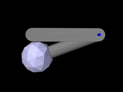
A model illustrating how to redefine the collision mesh for a rigid body is defined in
artisynth.demos.tutorial.JointedBallCollide
Like JointedCollide in Section 8.1.3, this model is simply a subclass of RigidBodyJoint that overrides the build() method, adding a ball to the tip of bodyA to enable it to collide with bodyB:
The superclass build() method called at line 3 creates everything contained in RigidBodyJoint. The remaining code then alters that model: A ball mesh is created, translated to the tip of bodyA, added as an additional mesh (Section 3.2.9), and set to render as blue-gray (lines 5-10). Next, collisions are disabled for bodyA’s main surface mesh by setting its isCollidable property to false (line 13); this will ensure that the collision mesh associated with bodyA will consist solely of the ball mesh, which is necessary because the surface mesh is permanently in contact with bodyB. Lastly, collisions are enabled between bodyA and bodyB (line 15).
To run this example in ArtiSynth, select All demos > tutorial > JointedBallCollide from the Models menu. Running the model will cause bodyA to fall, pivot about the hinge joint, and collide with bodyB (Figure 8.3).
8.3.2 Compound collidables and self-collision
An FEM model is an example of a compound collidable, which may contain subcollidable descendant components which are also collidable. Compound collidables are identified by having their isCompound() method return true. For an FEM model, the subcollidables are the mesh components in its meshes list. A non-compound collidable which is not a subcollidable of some other (compound) collidable is called solitary. If A is a subcollidable of a compound collidable C, then C is an ancestor collidable of A.
Subcollidables do not need to be immediate child components of the compound collidable; they need only be descendants.
One of the main purposes of compound collidables is to enable self-collisions. While ArtiSynth does not currently support the detection of self-collisions within a single mesh, self-collision can be implemented within a compound collidable C by detecting collisions among the (separate) meshes of its subcollidables.
Compound collidables and their subcollidables are assumed to be deformable; otherwise, subcollision would not be possible.
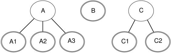
In general, an ArtiSynth model will contain a number of collidable components, some of which are compound (Figure 8.4). The non-compound collidables, including both solitary collidables and leaf nodes of a compound collidable’s tree, are also instances of the subinterface CollidableBody, which provide the collision meshes, along with other information used to compute the collision response (Section 8.3.4).
Actual collisions happen only between CollidableBodys; compound collidables are used only for determining grouping and specifying collision behaviors. The rules for determining whether two collidable bodies A and B will actually collide are as follows:
-
1.
Internal (self) collisions: If A and B are both subcollidables of some compound collidable C, then A and B will collide if (a) both their collidable properties are set to either ALL or INTERNAL, and (b) an explicit collision behavior is set between A and B, or self-collision is enabled for C (as described below).
-
2.
External collisions: Otherwise, if A and B are either solitary or subcollidables of different compound collidables, then they will collide if (a) both their collidable properties are set to either ALL or EXTERNAL, and (b) a specific or default collision behavior is set between them or their collidable ancestors.
As mentioned above, the subcollidables of an FEM are its mesh components (Section 6.3), each of which is a collidable implemented by FemMeshComp. When a mesh component is added to an FEM model, using either addMeshComp() or one of the addMesh() methods, its collidable property is automatically set to INTERNAL, so if a different setting is required, this must be specified after the component has been added to the model.
Subject to the above conditions, self-collision can be enabled for a specific compound collidable C by calling the setCollisionBehavior() methods with collidable0 set to C and collidable1 set to either C or Collidable.SELF, as in for example:
It can also be enabled, by default, for all compound collidables by calling one of the setDefaultCollisionBehavior() methods with collidable0 set to Collidable.DEFORMABLE and collidable1 set to Collidable.SELF, e.g.:
For an example of how collision interactions can be set, refer to Figure 8.4, assume that components A, B and C are deformable, and that the collidable property for all collidables is set to ALL except for A3, where it is set to EXTERNAL (implying that A3 cannot self-collide with A1 and A2). Then if mech is the MechModel containing the collidables, the call
will enable collisions between A1, A2, and A3 and each of B, C1, and C2, and between B and C1 and C2, but not among A1, A2, and A3 or C1 and C2. The subsequent calls
will enable self-collision between A1 and A2 and C1 and C2 with zero friction, and disable collision between B and A3. Finally, the calls
will enable collision between A3 and each of C1 and C2 with friction 0.3, and disable all self-collisions among A1, A2 and A3.
8.3.3 Example: FEM model with self-collision
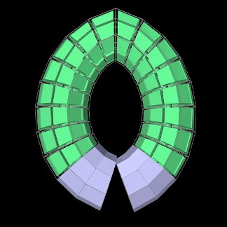 |
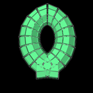 |
A model illustrating self-collision for an FEM model is defined in
artisynth.demos.tutorial.FemSelfCollide
It creates a simple FEM based on a partial torus that self intersects when it falls under gravity. Internal surface meshes are added to the left and right ends of the model to prevent interpenetration. The code for the build() method is listed below:
The model creates an FEM model based on an open torus, using a factory
method in FemFactory, and
rotates it so that the gap is located at the bottom (lines 7-18). The
torus is then anchored by fixing the nodes located at the top-center
(lines 20-25). Next, mesh components are created to enforce
self-collision at the left and right gap end points (lines 27-47).
First, a FemMeshComp is created
(Section 6.3), and then its createVolumetricSurface() method is used to create a local surface
mesh wrapping the elements specified in elems. When selecting
the elements, we use the convenient fact that for this particular FEM
model, the elements near the left and right ends have numbers in the
ranges ![]() and
and ![]() , respectively.
, respectively.
Once the submeshes have been added to the FEM model, we create a collision behavior and use it to enable self-collisions (lines 49-55). An explicit behavior is created so that we can enable the VERTEX_EDGE_PENETRATION contact method (Section 8.4.1), because the meshes are coarse and the additional edge-edge collisions will improve behavior; this method also requires the AJL_CONTOUR collider type. While self-collision is enabled by calling
it could also have been enabled by calling
Note that there is no need to set the collidable property of the collision meshes since it is set to INTERNAL by default when they are added to the FEM model.
Render properties are set at lines 57-64, with the torus rendered as light green and the collision meshes as blue-gray. The torus is drawn using its element widgets instead of its surface mesh, to prevent the latter from obscuring the collision meshes.
To run this example in ArtiSynth, select All demos > tutorial > FemSelfCollide from the Models menu. Running the model will cause the FEM model to self-collide as shown in Figure 8.5.
8.3.4 Collidable bodies
As mentioned in Section 8.3.2, non-compound collidables, including both solitary collidables and leaf nodes of a compound collidable’s tree, are also instances of CollidableBody, which provide the actual collision meshes and other information used to compute the collision response. This is done using various methods, including:
-
•
PolygonalMesh getCollisionMesh()
Returns the actual surface mesh to be used for computing collisions.
-
•
boolean hasDistanceGrid()
If this method returns true, the body also maintains a signed distance grid for the mesh, which can be used by the collider type SIGNED_DISTANCE (Section 8.4.1).
-
•
DistanceGridComp getDistanceGridComp()
If hasDistanceGrid() returns true, this method returns the distance grid.
-
•
double getMass()
Returns the mass of this body (or a suitable estimate), for use in automatically computing certain collision parameters.
-
•
int getCollidableIndex()
Returns the index of this collidable body within the set of all CollidableBodys in the MechModel. The index is determined by the body’s depth-first ordering within the model component hierarchy. For components within the same component list, this ordering will be determined by the order in which the components are added in the model’s build() method.
8.3.5 Nested MechModels
It is possible in ArtiSynth for one MechModel to contain other nested MechModels within its component hierarchy. This raises the question of how collisions within the nested models are controlled. The general rule for this is the following:
The collision behavior for two collidables colA and colB is determined by whatever behavior (either default or override) is specified by the lowest MechModel in the component hierarchy that contains both colA and colB.
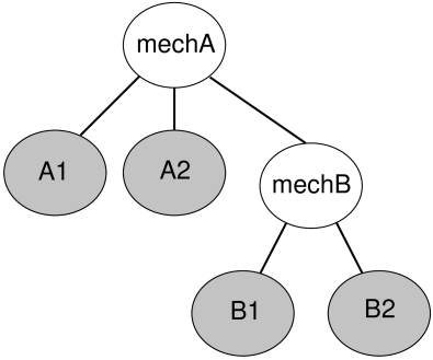
For example, consider Figure 8.6 where we have a MechModel (mechB) containing collidables B1 and B2, nested within another MechModel (mechA) containing collidables A1 and A2. Then consider the following code fragment:
The first line enables default collisions within mechB (with
![]() ), controlling the interaction between B1 and B2.
However, collisions are still disabled within mechA, meaning
A1 and A2 will not collide either with each other or with
B1 or B2. The second line enables collisions between B1 and any other body within mechA (i.e., A1 and
A2), while the third line disables collisions between B1
and A1. Finally, the fourth line results in an error, since
B1 and B2 are both contained within mechB and so
their collision behavior cannot be controlled from mechA.
), controlling the interaction between B1 and B2.
However, collisions are still disabled within mechA, meaning
A1 and A2 will not collide either with each other or with
B1 or B2. The second line enables collisions between B1 and any other body within mechA (i.e., A1 and
A2), while the third line disables collisions between B1
and A1. Finally, the fourth line results in an error, since
B1 and B2 are both contained within mechB and so
their collision behavior cannot be controlled from mechA.
While it is not legal to specify a specific behavior for collidables contained in a MechModel from a higher level MechModel, it is legal to create collision response components for the same pair within both models. So the following code fragment would be allowed and would create response components in both mechA and mechB:
8.4 Implementation
This section describes the technical details of the different ways in which collisions are implemented in ArtiSynth. Knowledge of these details can be useful for choosing collision behavior property settings, understanding elastic foundation contact (Section 8.7.3), and interpreting the information provided by collision responses (Section 8.8.1) and collision rendering (Section 8.5).
The collision mechanism works by using a collider (described further below) to locate the contact regions where the (triangular) collision meshes of different collidables intersect each other. Figure 8.7 shows four contact regions between two meshes representing human teeth. Information about each contact region is then used to generate contact constraints, according to a contact method, that prevent further collision and resolve any existing interpenetration.
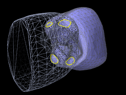
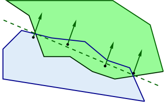 |
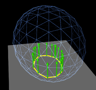 |
8.4.1 Contact methods
Contact constraints are computed from mesh contact regions using one of two primary contact methods:
8.4.1.1 Contour region
Contact constraints are generated for each contact region by first fitting a plane to the region, and then selecting contact points around its perimeter such that their 2D projection into the plane forms a convex hull (Figure 8.8). A contact constraint is assigned to each contact point, with a constraint direction parallel to the plane normal and a penetration distance given by the maximum interpenetration of the region. Note that the contact points do not necessarily lie on the plane, but they all have the same normal and penetration distance.
This is the default method used between rigid bodies, since it does not depend on mesh resolution, and rigid body contact behavior depends only on the convex hull of the contacting regions. Since the number of contact constraints may exceed the number of degrees of freedom (DOF) of the contacting bodies, the constraints are supplied to the physics solver as unilateral constraints (Section 1.2.3). Using contact region constraints when one of the collidables is an FEM model will result in an error.
8.4.1.2 Vertex penetration
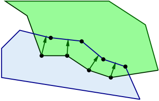 |
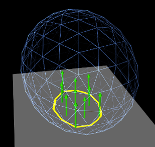 |
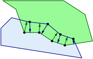
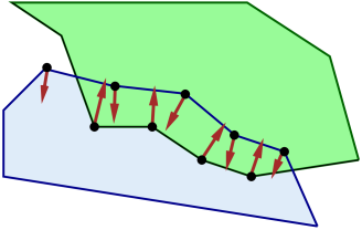
Contacts are created for each mesh vertex that penetrates the other mesh, with a contact normal directed toward the nearest point on the opposing mesh (Figure 8.9). Contact constraints are generated for each contact, with the constraint direction parallel to the normal and the penetration distance equal to the distance to the opposing mesh.
This is the default contact method when one or both of the collidables is an FEM model. Also by default, if only one of the collidables is an FEM model, vertex penetrations are computed only for the FEM collidable; penetrations of the rigid body into the FEM are not considered. Otherwise, if both collidables are FEM models, then vertex penetrations are computed for both bodies, resulting in two-way contact (Figure 8.10).
Vertex penetration contact results in contact reaction forces being generated on the mesh vertices that are within or next to the intersection region (Figure 8.9). These appear on vertices of both intersecting meshes, regardless of whether contact points are generated for one or both meshes, since each vertex associated with a contact imparts a reaction force on the vertices of the nearest face on the opposite mesh.
Because FEM models tend to have a large number of DOFs, the default behavior is to supply vertex penetration constraints to the physics solver as bilateral constraints (Section 1.2.3), removing them only between simulation time steps when the contact disappears or a separating force is detected. This results in much faster simulation times, particularly for FEM models, because it does not require solving a linear complementarity problem. However, this also means that using vertex penetration between rigid bodies, or other bodies with a low number of degrees of freedom, will typically result in an overconstrained system that must be handled using one of the techniques described in Section 8.6.
8.4.1.3 Setting the contact method
Contact methods can be specified by the method property in either the collision manager or behavior (Section 8.2.1). The property’s value is an instance of CollisionBehavior.Method, for which the standard settings are:
- CONTOUR_REGION
-
Contact constraints are generated using contour regions, as described in Section 8.4.1.1. Setting this for contact that involves one or more FEM models will result in an error.
- VERTEX_PENETRATION
-
Contact constraints are generated using vertex penetration, as described in Section 8.4.1.2. Setting this for contact between rigid bodies may result in an overconstrained system.
- VERTEX_EDGE_PENETRATION
-
An experimental version of vertex penetration contact that supplements vertex constraints with extra constraints formed from edge-edge contact. Intended for collision meshes with low mesh resolutions and sharp edges. Available only when using the AJL_CONTOUR collider type (Section 8.4.2).
- DEFAULT
-
Selects CONTOUR_REGION when both collidables are rigid bodies and VERTEX_PENETRATION otherwise.
- INACTIVE
-
No constraints are generated. This will result in no collision response.
When vertex penetration contact is employed, the collidables for which penetrations are generated can also be controlled using the vertexPenetrations property, whose value is an instance of CollisionBehavior.VertexPenetrations:
- BOTH_COLLIDABLES
-
Vertex penetrations are computed for both collidables.
- FIRST_COLLIDABLE
-
Vertex penetrations are computed for the first collidable.
- SECOND_COLLIDABLE
-
Vertex penetrations are computed for the second collidable.
- AUTO
-
Vertex penetrations are determined automatically as follows: for both collidables if neither is a rigid body, for the non-rigid collidable if one collidable is a rigid body, and for the first collidable otherwise.
8.4.2 Collider types
The contact regions used by the contact method are generated by a collider, which is specified by the colliderType property in either the collision manager (as the default), or in the collision behavior for a specific pair of collidables. The property’s value is an instance of CollisionManager.ColliderType, which describes the three collider types presently supported:
- TRI_INTERSECTION
-
The original ArtiSynth collider which uses a bounding-box hierarchy to locate all triangle intersections between the two surface meshes. Contact regions are then estimated by grouping the intersection points together, and penetrating vertices are computed separately using point-mesh distance queries based on the bounding-box hierarchy. This latter step requires iterating over all mesh vertices, which may be slow for large meshes. TRI_INTERSECTION can often handle intersections near the edges of an open mesh, but does not support the VERTEX_EDGE_PENETRATION contact method.
- AJL_CONTOUR
-
A bounding-box hierarchy is used to locate all triangle intersections between the two surface meshes, and the intersection points are then connected, using robust geometric predicates, to find the (piecewise linear) intersection contours. The contours are then used to identify the contact regions on each surface mesh, which are in turn used to determine the interpenetrating vertices and contact area. Intersection contours and the contact constraints generated from them are shown in Figure 8.12. AJL_CONTOUR supports the VERTEX_EDGE_PENETRATION contact method, but usually cannot handle intersections near the edges of an open mesh.
- SIGNED_DISTANCE
-
Uses a grid-based signed distance field on one mesh to quickly determine the penetrating vertices of the opposite mesh, along with the penetration distance and normals. This is only available for collidable pairs where at least one of the bodies maintains a signed distance grid which can be obtained using getDistanceGridComp(). Advantages include speed (sometimes an order of magnitude faster than the other colliders) and the fact that the opposite mesh does not have to be triangular or manifold. However, signed distance fields can (at present) only be computed for fixed meshes, and so at least one colliding body must be rigid. The signed distance field also does not yet yield contact region information, and so the contact method is restricted to VERTEX_PENETRATION. Contacts generated from a signed distance field are illustrated in Figure 8.13.
Because the SIGNED_DISTANCE collider type currently supports only the VERTEX_PENETRATION method, its use between rigid bodies, or low DOF deformable bodies, will generally result in an overconstrained system unless measures are taken as described in Section 8.6.
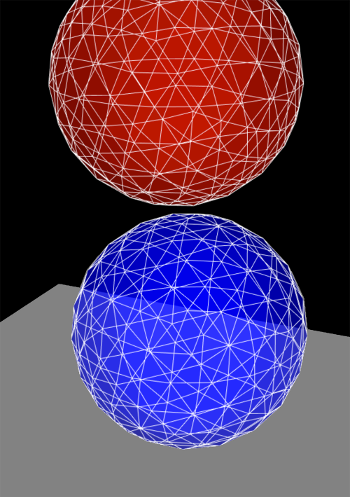 |
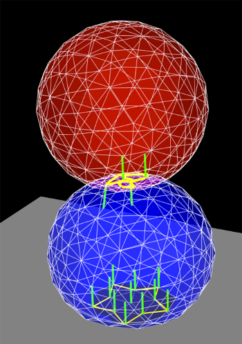 |
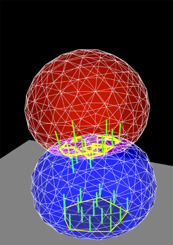 |
|
|
|
|
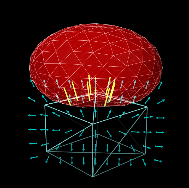
8.4.2.1 Collision meshes and signed distance grids
As described in Section 8.3.4, collidable bodies declare the method getCollisionMesh(), which returns a mesh defining the collision surface. This is either used directly, or, for the SIGNED_DISTANCE collider, used to compute a signed distance grid which in turn is used to handle collisions.
For RigidBody objects, the mesh returned by getCollisionMesh() is typically the same as the surface mesh. However, it is possible to change this, by adding additional meshes to the body and modifying the meshes’ isCollidable property (see Section 8.3). The collision mesh is then formed as the sum of all polygonal meshes in the body’s meshes list whose isCollidable property is true.
Collidable bodies also declare the methods hasDistanceGrid() and getDistanceGridComp(). If the former returns true, then the body has a distance grid and the latter returns a DistanceGridComp containing it. A distance grid is a regular 3D grid, with uniformly arranged vertices and cells, that is used to represent a scalar distance field, with distance values stored implicitly at each vertex and interpolated within cells. Distance grids are used by the SIGNED_DISTANCE collider, and by default are generated on-demand, using an automatically chosen resolution and the mesh returned by getCollisionMesh() as the surface against which distances are computed.
When used for collision handling, values within a distance grid are interpolated trilinearly within each cell. This means that the effective collision surface is actually the trilinearly interpolated isosurface corresponding to a distance of 0. This surface will differ somewhat from the original surface returned by getCollisionMesh(), in a manner that depends on the grid resolution. Consequently, when using the SIGNED_DISTANCE collider, it is important to be able to visualize the trilinear isosurface, and possibly modify it by adjusting the grid resolution. The DistanceGridComp returned by getDistanceGridComp() exports properties to facilitate both of these requirements, as described in detail in Section 4.6.
8.5 Contact rendering
As mentioned in Section 8.2.1, additional collision behavior properties exist to enable and control the rendering of contact artifacts. These include intersection contours, contact points and normals, contact forces and pressures, and penetration depths. The properties that control these are supplemented by generic render properties (Section 4.3) to specify colors, line widths, etc.
By default, contact rendering is disabled. To enable it, one must set the collision manager to be visible, which can be done using a code fragment like the following:
RenderProps.setVisible (mechModel.getCollisionManager(), true);
CollisionManager and CollisionBehavior both export contact rendering properties. Setting these in the former controls rendering globally for all collisions, while setting them in the latter controls rendering for the collidable pair associated with the behavior. Some artifacts, like contact normals, forces, and color maps, must be drawn with respect to either the first or second collidable. By default, the first collidable is chosen, but the second collidable can be requested using the renderingCollidable property described below. Normals are drawn toward, and forces drawn such that they are acting on, the indicated collidable. For collision behaviors specified using the setCollisionBehavior() methods, the first and second collidables correspond to the collidable0 and collidable1 arguments. Otherwise, for default collision behaviors, the first collidable will be the one whose collidable bodies have the lowest collidable index (Section 8.3.4).
Properties exported by both CollisionManager and CollisionBehavior include:
- renderingCollidable
-
Integer value of either 0 or 1 specifying the collidable for which forces, normals and color maps should be drawn. 0 or 1 selects either the first or second collidable. The default value is 0.
- drawIntersectionContours
-
Boolean value requesting drawing of the intersection contours between collidable meshes, using the generic render properties edgeWidth and edgeColor. The default value is false.
- drawIntersectionPoints
-
Boolean value requesting drawing of the interpenetrating vertices on each collidable mesh, using the generic render properties pointStyle, pointSize, pointRadius, and pointColor. The default value is false.
- drawContactNormals
-
Boolean value requesting drawing of the normals associated with each contact constraint, using the generic render properties lineStyle, lineRadius, lineWidth, and lineColor. The default value is false. The length of the normals is controlled by the contactNormalLen property of the collision manager, which will be set to an appropriate default value if not set explicitly.
- drawContactForces
-
Boolean value requesting drawing of the forces associated with each contact constraint, using the generic render properties lineStyle, lineRadius, edgeWidth, and edgeColor (or lineColor if edgeColor is null). The default value is false. The forces are drawn as line segments starting at each contact point and running parallel to the contact normal, with a length given by the current contact impulse value multiplied by the contactForceLenScale property of the collision manager (which has a default value of 1). The reason for using edgeWidth and edgeColor instead of lineWidth and lineColor is to allow the application to set the render properties such that both normals and forces can be visible if both are being rendered at the same time.
- drawFrictionForces
-
Boolean value requesting the drawing of the forces associated with each contact’s friction force, in the same manner and style as for drawContactForces. The default value is false. Note that unlike contact forces, friction forces are perpendicular to the contact normal.
- drawColorMap
-
An enum of type CollisionBehavior.ColorMapType requesting that a color map be drawn over the contact regions showing a scalar value such as penetration depth or contact force pressure. The collidable (0 or 1) onto which the color map is drawn is controlled by the renderingCollidable property (described below). The range of values used for generating the map is controlled by the colorMapRange property of either the collision manager or the behavior, as described below. The values are mapped onto colors using the colorMap property of the collision manager.
Values of CollisionBehavior.ColorMapType include:
- NONE
-
The color map is disabled. This is the default value.
- PENETRATION_DEPTH
-
The color map shows penetration depth of one collidable mesh with respect to the other. If one or both collidable meshes are open, then the colliderType should be set to AJL_CONTOUR (Section 8.2.1).
- CONTACT_PRESSURE
-
The color map shows the contact pressures over the contact region. Contact pressures are determined by examining the forces at the contact constraints and then distributing these over the surrounding faces. This information is most useful and accurate when using vertex penetration contact (Section 8.4.1.2).
The color map itself is drawn as a patch formed from the collidable’s collision mesh, using faces and vertices associated with the collision region. The vertices of the patch are set to colors corresponding to the associated value (e.g., penetration depth or pressure) at that vertex, and the surrounding faces are colored appropriately. The resolution of the color map is thus determined by the resolution of the collision mesh, and so the application must ensure this is high enough to ensure proper results. If the mesh has only a few triangles (e.g., a rectangle with two triangles per face), the color interpolation may be spread over an unreasonably large area. Examples of color map usage are given in Sections 8.5.2 and 8.5.3.
- colorMapRange
-
Composite property of the type ScalarRange that controls the range of values used for color map rendering. Subproperties include interval, which gives the value range itself, and updating, which specifies how this interval should be updated: FIXED (no updating), AUTO_EXPAND (interval is expanded as values increase or decrease), and AUTO_FIT (interval is reset to fit the values at every render step).
When the colorMapRange value for a CollisionBehavior is set to null (which is the default), the colorMapRange of the CollisionManager is used instead. This has the advantage of ensuring that the same color map range will be used across all collision interactions.
- colorMapInterpolation
-
An enum of type Renderer.ColorInterpolation that explicitly specifies how colors in any rendered color map should be interpolated. RGB and HSV (the default) specify interpolation in RGB and HSV space, respectively. HSV interpolation is the default as it is generally better suited to rendering maps that are purely color-based.
In addition, the following properties are exported by the collision manager:
- contactNormalLen
-
Double value specifying the length with which contact normals should be drawn when drawContactNormals is true. If unspecified, a default value is calculated by the system.
- contactForceLenScale
-
Double value specifying the scaling factor for contact or friction force vectors when they are drawn in response to drawContactForces or drawFrictionForces being true. The default value is 0.
- colorMap
-
Composite property of type ColorMapBase specifying the actual color map used for color map rendering. The default value is HueColorMap.
Generic render properties within the collision manager can be set in the same way as the visibility, using the RenderProps methods presented in Section 4.3.2:
As mentioned above, generic render properties can also be set individually for specific behaviors. This can be done using code fragments like this:
To access these properties on a read-only basis, one can do
Because of the manner in which ArtiSynth handles contacts, rendered contact information may sometimes appear to lag the simulation by one time step. That is because contacts are computed at the end of each time step
, and then used to compute the contact forces during the next step
. The contact information displayed at the end of step
, along with contact forces that are computed during step
8.5.1 Example: rendering normals and contours
A simple model illustrating contact rendering is defined in
artisynth.demos.tutorial.BallPlateCollide
This shows a ball colliding with a plate, while rendering the resulting contact normals in red and the intersection contours in blue. This demo also allows the user to experiment with compliant contact (Section 8.7.1) by setting compliance and damping properties in a control panel.
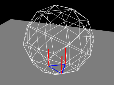
The complete source code is shown below:
The build() method starts by creating and adding a MechModel in the usual way (lines 19-20). The ball and plate are both created as rigid bodies (lines 22-28), with the ball pose set so that its origin is above the plate at (0, 0, 2) and its orientation is perturbed so that it will not land on the plate symmetrically (line 24). Collisions between the ball and plate are enabled at line 31, with a friction coefficient of 0.2. To allow better visualization of the contacts, the ball is made transparent by disabling the drawing of faces, and instead enabling the drawing of edges in white with no shading (lines 33-37).
Rendering of contacts and normals is established by setting the render properties of the collision manager (lines 39-47). First, the collision manager is set visible (which it is not by default). Then lines (used to render the contact normals) and edges (used to render to intersection contour) are set to red and blue, each with a pixel width of 3. Drawing of the normals and contour is enabled at lines 46-47.
Lastly, for interactively controlling contact compliance (Section 8.7.1), a control panel is built to allow users to adjust the collision manager’s compliance and damping properties (lines 49-53).
To run this example in ArtiSynth, select All demos > tutorial > BallPlateCollide from the Models menu. When run, the ball will collide with the plate and the contact normals and collision contours will be drawn as shown in Figure 8.14.
To enable compliant contact, set the compliance to a
non-zero value. A value of 0.001 (which corresponds to a contact
stiffness of 1000) causes the ball to bounce considerably when it
lands. To counteract this bouncing, the damping should be set to
a non-zero value. Since the ball has a mass of 0.21, formula
(8.2) suggests that critical damping (for which
![]() ) can be achieved with
) can be achieved with ![]() . This does in fact stop
the bouncing. Increasing the compliance to 0.01 results in the ball
penetrating the plate by a noticeable amount.
. This does in fact stop
the bouncing. Increasing the compliance to 0.01 results in the ball
penetrating the plate by a noticeable amount.
8.5.2 Example: rendering a color map
As described above, it is possible to use the drawColorMap property of the collision behavior to render a color map over the contact area showing a scalar value such as penetration depth or contact pressure. A simple example of this is defined in
artisynth.demos.tutorial.PenetrationRender
which sets drawColorMap to PENETRATION_DEPTH in order to display the penetration depth of one hemispherical mesh with respect to another.
As mentioned above, proper results require that the collision mesh for the collidable on which the map is being drawn has a sufficiently high resolution.
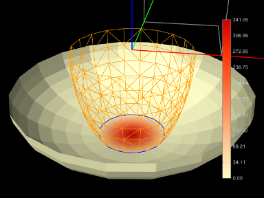
The complete source code is shown below:
To improve visibility, the example uses two rigid bodies, each created from an open hemispherical mesh using the method createHemiBody() (lines 32-47). Because this example is strictly graphical, the bodies are set to be non-dynamic so that they can be moved around using the viewer’s graphical dragger fixtures (see the section “Transformer Tools” in the ArtiSynth User Interface Guide). Rendering properties for each body are set at lines 67-68 and 73-76, with the top body being rendered as a wireframe to improve visibility.
Lines 80-84 create and set a collision behavior between the two bodies with the drawColorMap property set to PENETRATION_DEPTH. Because for this example we want to show only the penetration and don’t want a collision response, we set the contact method to be Method.INACTIVE. At line 88, the collider type used by the collision manager is set to ColliderType.AJL_CONTOUR, since this provides more reliable penetration calculations for open meshes. Other rendering properties are set for the collision manager at lines 90-107, including a custom color map that varies between CREAM (the color of the mesh) for no penetration and dark red for maximum penetration. The updating of the color map range in the collision manager is set to AUTO_FIT so that it will be recomputed at every time step. (Since the collision manager’s color map range is set to “auto fit” by default, this is shown for illustrative purposes only. It is also possible to override the collision manager’s color map range by setting the colorMapRange property in specific collision behaviors.)
At line 111, a color bar is created and added to the scene, using the method createColorBar() (lines 50-59), to explicitly show the depth that corresponds to the different colors. The color bar is given the same color map that is used to render the depth. Since the depth range is updated every time step, it is also necessary to update the corresponding labels in the color bar. This is done by overriding the root model’s prerender() method (lines 115-132), where we obtain the color map range for the collision manager and use it to update the color bar labels. (Note that super.prerender(list) is called first, since the color map ranges are updated there.) References to the color bar, MechModel, and bodies are obtained using the CompositeComponent methods get() and findComponent(). This is more robust than storing these references in member variables, since the latter would be lost if the model is saved to and reloaded from a file.
To run this example in ArtiSynth, select All demos > tutorial > PenetrationRender from the Models menu. When run, the meshes will collide and render the penetration depth of the bottom mesh, as shown in Figure 8.15.
When defining the color map for rendering (lines 99-108 in the example), it is recommended that the color corresponding to zero be set to the face color of the collidable mesh. This will allow the color map to blend properly to the regular mesh color.
8.5.3 Example: rendering contact pressures
Color map rendering can also be used to render contact pressures, which can be particularly useful for FEM models. A simple example is defined in
artisynth.demos.tutorial.ContactPressureRender
which sets the drawColorMap property of the collision behavior to CONTACT_PRESSURE in order to display a color map of the contact pressure. The example is similar to that of Section 8.5.2, which shows how to render penetration depth.
The caveats about color map rendering described in Section 8.5 apply. Pressure rendering is most useful and accurate when using vertex penetration contact. The resolution of the color map is limited by the resolution of the collision mesh for the collidable on which the map is drawn, and so the application should ensure that this is sufficiently fine. Also, to allow the map to blend properly with the rest of the collidable, the color corresponding to zero pressure should match the default face color for the collidable.
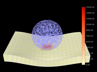
The complete source code is shown below:
To begin, the demo creates two FEM models: a spherical ball (lines 52-56) and a rectangular sheet (lines 59-66), and then fixes the end nodes of the sheet (lines 69-74). Surface rendering is enabled for the sheet (line 65), but not for the ball, in order to improve the visibility of the color map.
Lines 77-81 create and set a collision behavior between the two
models, with the drawColorMap property set to CONTACT_PRESSURE. Because for this example we want the color map to
be drawn on the second collidable (the sheet), we set the renderingCollidable property to 1 (line 79); otherwise, the default
value of 0 would cause the color map to be drawn on the first
collidable (the ball). (Alternatively, we could have simply defined
the collision behavior as being between the surface and the ball
instead of the ball and the sheet.) The color map range is explicitly
set to lie between ![]() (line 80); this is in contrast to the
example in Section 8.5.2, where the range is
auto-updated on each step. The color range is also set explicitly in
the behavior, but if multiple objects were colliding it would likely
be preferable to set it in the collision manager (with the behavior’s
value left as null) to ensure a uniform render range across all
collisions. Other rendering properties are set for the collision
manager at lines 83-97, including a custom color map that varies
between CREAM (the color of the mesh) for no pressure and dark
red for maximum pressure.
(line 80); this is in contrast to the
example in Section 8.5.2, where the range is
auto-updated on each step. The color range is also set explicitly in
the behavior, but if multiple objects were colliding it would likely
be preferable to set it in the collision manager (with the behavior’s
value left as null) to ensure a uniform render range across all
collisions. Other rendering properties are set for the collision
manager at lines 83-97, including a custom color map that varies
between CREAM (the color of the mesh) for no pressure and dark
red for maximum pressure.
At line 100, a color bar is created and added to the scene, using the method createColorBar() (lines 36-45), to explicitly show the pressure that corresponds to the different colors. The color bar is given the same color map and value range used to render the pressure. Finally, default face and line colors for all components in the model are set at lines 105-106.
To run this example in ArtiSynth, select All demos > tutorial > ContactPressureRender from the Models menu. When run, the FEM models will collide and render the contact pressure on the sheet, as shown in Figure 8.16.
8.6 Overconstrained contact
When contact occurs between collidable bodies, the system creates a set of contact constraints to handle the collision and passes these to the physics solver (Section 1.2.3). When one or both of the contacting collidables are FEM models, the number of constraints is usually less than the DOF count of the collidables. However, if the both collidables are rigid bodies, then the number of constraints often exceeds the DOF count, a situation which is referred to as redundant contact. Redundant contact can also occur in other collision situations, such those involving embedded meshes (Section 6.3.2) when the mesh has a finer resolution than the embedding FEM, or skinned meshes (Chapter 11) when the number of contacts exceeds the DOF count of the underlying master bodies.
Redundant contact is not usually a problem in collisions between rigid bodies, because by default ArtiSynth handles these using CONTOUR_REGION contact (Section 8.4.1), for which contacts are supplied to the physics solver as unilateral constraints which are solved using complementarity techniques that can handle redundant constraints. However, as mentioned in Section 8.4.1.2, the default implementation for vertex penetration contact is to present the contacts to the physics solver as bilateral constraints (Section 1.2.3), which are removed between simulation steps. This results in much faster simulation times, and usually works well in the case of FEM models, where the DOF count almost always exceeds the number of constraints. However, when vertex penetration contact is employed between rigid bodies, and sometimes in other situations as described above, redundant contact can arise, and then the use of bilateral constraints results in overconstrained contact for which the solver has difficulty finding a proper solution.
A common indicator of overconstrained contact is for an error message to appear in ArtiSynth’s console output, which typically looks like this:
Pardiso: num perturbed pivots=12
The simulation may also go unstable.
At present there are three general ways to manage overconstrained contact:
-
1.
Requiring the system to use unilateral constraints for vertex penetration contact. This can be done by setting the property bilateralVertexContact (Section 8.2.1) to false in either the collision manager or behavior, but the resulting hit to computational performance may be large.
-
2.
Constraint reduction, described in Section 8.6.1.
-
3.
Regularizing the contact, using one of the methods of Section 8.7.
When using the new implicit friction integration feature (Section 8.9.4), if redundant contacts arise, it is necessary to regularize both the contact constraints, as per Section 8.7, as well as the friction constraints, by setting the stictionCreep property of either the collision manager or behavior to a non-zero value, as described in Section 8.2.1.
8.6.1 Constraint reduction
Constraint reduction involves having the collision manager explicitly try to reduce the number of collision constraints to match the available DOFs, and is enabled by setting the reduceConstraints property for either the collision manager or the CollisionBehavior for a particular collision pair to true. The default value of reduceConstraints is false. As with all properties, it can be set interactively in the GUI, or in code using the property’s accessor methods,
as illustrated by the following code fragments:
8.7 Contact regularization
Contact regularization is a technique in which contact constraints are made “soft” by adding compliance and damping. This means that they no longer remove DOFs from the system, and so overconstraining cannot occur, but contact penetration is no longer strictly enforced and there may be an increase in the computation time required for the simulation.
8.7.1 Compliant contact
Compliant contact is a simple form of regularization that is analogous
to that used for joints and connectors, discussed in Section
3.4.9. Compliance and damping parameters ![]() and
and
![]() can be specified between any two collidables, with
can be specified between any two collidables, with ![]() being the
inverse of a corresponding contact stiffness
being the
inverse of a corresponding contact stiffness ![]() , such the
contact forces
, such the
contact forces ![]() acting along each contact normal are given by
acting along each contact normal are given by
| (8.1) |
where ![]() is the contact penetration distance and is negative
when penetration occurs. Contact forces act to push the contacting
bodies apart, so if body A is penetrating body B and the contact
normal
is the contact penetration distance and is negative
when penetration occurs. Contact forces act to push the contacting
bodies apart, so if body A is penetrating body B and the contact
normal ![]() is directed toward A, the forces acting on A and B
at the contact point will be
is directed toward A, the forces acting on A and B
at the contact point will be ![]() and
and ![]() , respectively.
Since
, respectively.
Since ![]() is the inverse of the contact stiffness
is the inverse of the contact stiffness ![]() , a value of
, a value of ![]() (the default) implies “infinitely” stiff contact
constraints. Compliance is enabled whenever the compliance is set
to a value greater than 0, with stiffness decreasing as compliance
increases.
(the default) implies “infinitely” stiff contact
constraints. Compliance is enabled whenever the compliance is set
to a value greater than 0, with stiffness decreasing as compliance
increases.
Compliance can be enabled by setting the compliance and damping properties of either the collision manager or the
CollisionBehavior for a
specific collision pair; these properties correspond to ![]() and
and ![]() in
(8.1). While it is not required to set the damping
property, it is usually desirable to set it to a value that
approximates critical damping in order to prevent “bouncing” contact
behavior. Compliance and damping can be set in the GUI by editing the
properties of either the collision manager or a specific collision
behavior, or set in code using the accessor methods
in
(8.1). While it is not required to set the damping
property, it is usually desirable to set it to a value that
approximates critical damping in order to prevent “bouncing” contact
behavior. Compliance and damping can be set in the GUI by editing the
properties of either the collision manager or a specific collision
behavior, or set in code using the accessor methods
as is illustrated by the following code fragments:
An important question is what values to choose for compliance and
damping. At present, there is no automatic way to determine these, and
so some experimental parameter tuning is often necessary. With regard
to the contact stiffness ![]() , appropriate values will depend on the
desired maximum penetration depth and other loadings acting on the
body. The mass of the collidable bodies may also be relevant if one
wants to control how fast the contact stabilizes. (The mass of every
CollidableBody can be
determined by its getMass() method.) Since
, appropriate values will depend on the
desired maximum penetration depth and other loadings acting on the
body. The mass of the collidable bodies may also be relevant if one
wants to control how fast the contact stabilizes. (The mass of every
CollidableBody can be
determined by its getMass() method.) Since ![]() acts on a
per-contact basis, the resulting total force will increase with the
number of contacts. Once
acts on a
per-contact basis, the resulting total force will increase with the
number of contacts. Once ![]() is determined, the compliance value
is determined, the compliance value ![]() is simply the inverse:
is simply the inverse: ![]() .
.
Given ![]() , the damping
, the damping ![]() can then be estimated based on the desired
damping ratio
can then be estimated based on the desired
damping ratio ![]() , using the formula
, using the formula
| (8.2) |
where ![]() is the combined mass of the collidable bodies (or the mass
of one body if the other is non-dynamic). Typically, the desired
damping will be close to critical damping, for which
is the combined mass of the collidable bodies (or the mass
of one body if the other is non-dynamic). Typically, the desired
damping will be close to critical damping, for which ![]() .
.
An example that allows a user to play with contact regularization is given in Section 8.5.1.
8.7.2 Contact force behaviors
When regularizing contact through compliance, as described in
Section 8.6, the forces ![]() at each
contact are explicitly determined as per (8.1). As
a broader alternative to this, ArtiSynth allows applications to
specify a contact force behavior,
which allows
at each
contact are explicitly determined as per (8.1). As
a broader alternative to this, ArtiSynth allows applications to
specify a contact force behavior,
which allows ![]() to be computed as a more generalized function of
to be computed as a more generalized function of
![]() :
:
| (8.3) |
where ![]() and
and ![]() are functions returning the elastic force and
the damping coefficient. The corresponding compliance is then a local
function of
are functions returning the elastic force and
the damping coefficient. The corresponding compliance is then a local
function of ![]() given by
given by ![]() (which is the inverse of the
local stiffness).
(which is the inverse of the
local stiffness).
Because
should also be negative.
, on the other hand, should be positive, so that the damping acts to reduce
.
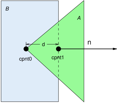
Contact force behaviors are implemented as subclasses of the abstract class ContactForceBehavior. To enable them, the application sets the forceBehavior property of the CollisionBehavior controlling the contact interaction, using the method
A ContactForceBehavior must implement the method computeResponse() to compute the contact force, compliance and damping at each contact:
The arguments to this method supply specific information about the contact (see Figure 8.17):
- fres
-
An array of length three that returns the contact force, compliance and damping in its first, second and third entries. The contact force is the
shown in (8.3), the compliance
is  , and the damping is .
 - dist
-
The penetration distance
(the value of which is negative). - cpnt0, cpnt1
-
ContactPoint objects containing information about the two points associated with the contact (Figure 8.17), including each point’s position (returned by getPoint()) and associated vertices and weights (returned by numVertices(), getVertices(), and getWeights()).
- nrml
-
The contact normal
. - contactArea
-
Average area per contact, computed by dividing the total area of the contact region by the number of penetrating vertices. This information is only available if the colliderType property of the collision behavior is set to AJL_CONTOUR (Section 8.2.1); otherwise, contactArea will be set to -1.
A collision force behavior may use its computeResponse() method
to calculate the force, compliance and damping in any desired way. As
per equation (8.3), these quantities are
functions of the penetration distance ![]() , supplied by the argument
dist.
, supplied by the argument
dist.
A very simple instance of ContactForceBehavior that just recreates the contact compliance of (8.1) is shown below:
This example uses only the penetration distance information supplied by dist, dividing it by the compliance to determine the contact force. Since dist is negative when the collidables are interpenetrating, the returned contact force will also be negative.
8.7.2.1 Computing forces based on pressure
Often, such as when implementing elastic foundation contact
(Section 8.7.3), the contact force
behavior is expressed in terms of pressure, given as a
function of ![]() :
:
| (8.4) |
In that case, the contact force ![]() is determined by multiplying
is determined by multiplying
![]() by the local area
by the local area ![]() associated with the contact:
associated with the contact:
| (8.5) |
Since
is negative as well.
To find the area ![]() within the computeResponse() method, one
has two options:
within the computeResponse() method, one
has two options:
-
A)
Compute an estimate of the local contact area surrounding the contact, as discussed below. This may be the more appropriate option if the colliding mesh vertices are not uniformly spaced, or if the contactArea argument is undefined because the AJL_CONTOUR collider (Section 8.4.2) is not being used.
-
B)
Use the contactArea argument if it is defined. This gives an accurate estimate of the per-contact area on the assumption that the colliding mesh vertices are uniformly distributed. contactArea will be defined when using the AJL_CONTOUR collider (Section 8.4.2); otherwise, it will be set to -1.
For option (A), ContactForceBehavior provides the convenience method computeContactArea(cpnt0,cpnt1,nrml), which estimates the local contact area given the contact points and normal. If the above example of computeResponse() is modified so that the stiffness parameter controls pressure instead of force, then we obtain the following:
computeContactArea() only works for vertex penetration contact (Section 8.4.1.2), and will return -1 otherwise. That’s because it needs the contact points’ vertex information to compute the area. In particular, for vertex penetration contact, it associates the vertex with 1/3 of the area of each of its surrounding faces.
When computing contact forces, care must also be taken to consider whether the vertex penetrations are being computed for both colliding surfaces (two-way contact, Section 8.4.1.2). This means that forces are essentially being computed twice - once for each side of the penetrating surface. For forces based on pressure, the resulting contact forces should then be halved. To determine when two-way contact is in effect, the flags argument can be examined for the flag TWO_WAY_CONTACT:
8.7.3 Elastic foundation contact
ArtiSynth supplies a built-in contact force behavior, LinearElasticContact, that implements elastic foundation contact (EFC) based on a linear material law as described in [3]. By default, the contact pressures are computed from
| (8.6) |
where ![]() is Young’s modulus,
is Young’s modulus, ![]() is Poisson’s ratio,
is Poisson’s ratio, ![]() is the
contact penetration distance, and
is the
contact penetration distance, and ![]() is the foundation layer
thickness. (Note that both
is the foundation layer
thickness. (Note that both ![]() and
and ![]() are negated relative to the
formulation in [3] because we assume
are negated relative to the
formulation in [3] because we assume ![]() during
contact.) The use of the
during
contact.) The use of the ![]() function helps ensure that contact
does not penetrate the foundation layer. However, to ensure robustness
in case contact does penetrate the layer (or comes close to
doing so), the pressure relationship is linearized (with a steep
slope) whenever
function helps ensure that contact
does not penetrate the foundation layer. However, to ensure robustness
in case contact does penetrate the layer (or comes close to
doing so), the pressure relationship is linearized (with a steep
slope) whenever ![]() , where
, where ![]() is the minimum thickness
ratio controlled by the LinearElasticContact property minThicknessRatio.
is the minimum thickness
ratio controlled by the LinearElasticContact property minThicknessRatio.
Alternatively, if a strictly linear pressure relationship is desired, this can be achieved by setting the property useLogDistance to false. The pressure relationship then becomes
| (8.7) |
where again ![]() will be negative when
will be negative when ![]() .
.
Damping forces ![]() can be computed in one of two ways: either
with
can be computed in one of two ways: either
with ![]() set to a constant
set to a constant ![]() such that
such that
| (8.8) |
or with ![]() set to a multiple of
set to a multiple of ![]() and the magnitude of the
elastic contact force
and the magnitude of the
elastic contact force ![]() , such that
, such that
| (8.9) |
The latter is compatible with the EFC damping used by OpenSim (equation 24 in [22]).
Elastic foundation contact assumes the use of vertex penetration contact (Section 8.4.1) to achieve correct results; otherwise, a runtime error may result.
LinearElasticContact exports several properties to control the force response described above:
- youngsModulus
-
- poissonsRatio
-
- thickness
-
- minThicknessRatio
-
 value such that (8.6) is linearized if
 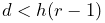 .
The default value is 0.01.
.
The default value is 0.01. - dampingFactor
-
- dampingMethod
-
An enum of type ElasticContactBase.DampingMethod, for which DIRECT and FORCE cause damping to be implemented using (8.8) and (8.9), respectively. The default value is DIRECT.
- useLogDistance
-
- useLocalContactArea
-
A boolean, which if true causes contact areas to be estimated from the vertex of the penetrating contact point (option A in Section 8.7.2.1). The default value is true.
8.7.4 Example: elastic foundation contact of a ball in a bowl
A simple example of elastic foundation contact is defined by the model
artisynth.demos.tutorial.ElasticFoundationContact
This implements EFC between a spherical ball and a bowl into which it is dropped. Pressure rendering is enabled (Section 8.5.3), and the bowl is made transparent, allowing the contact pressure to be viewed as the ball moves about.
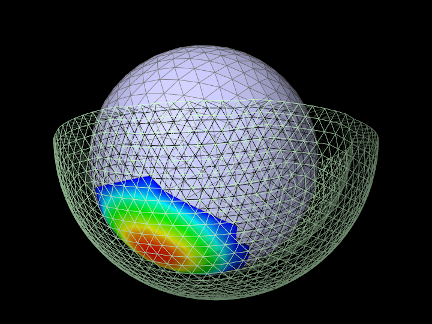
The source code for the build method is shown below:
The demo first creates the ball and the bowl as rigid bodies (lines 6-26), with the bowl defined by a mesh read from the file data/bowl.obj relative to the demo source directory, and the ball defined as an icosahedral sphere. The bowl is fixed in place (bowl.setDynamic(false)), and the ball is positioned at a suitable location for dropping into the bowl when simulation begins.
Next, a collision behavior is created, with its collision method
property set to VERTEX_PENETRATION (as required for EFC), and a
friction coefficient of 0.1 (to ensure that the ball will actually
roll) (lines 28-31). A LinearElasticContact is then constructed,
with ![]() ,
, ![]() , damping factor
, damping factor ![]() , and thickness
, and thickness ![]() ,
and added to the collision behavior using setForceBehavior()
(lines 32-26). The behavior is then used to enable contact between the
ball and bowl (line 39).
,
and added to the collision behavior using setForceBehavior()
(lines 32-26). The behavior is then used to enable contact between the
ball and bowl (line 39).
Lines 41-49 set up rendering properties: the collision manager is made visible, with color map rendering set to CONTACT_PRESSURE, and the ball and bowl are set to be rendered in pale blue and green, with the bowl rendered using only mesh edges so as to make it transparent.
Finally, a control panel is created allowing the user to adjust properties of the contact force behavior and the pressure rendering range (lines 51-57).
To run this example in ArtiSynth, select All demos > tutorial > ElasticFoundationContact from the Models menu. Running the model will cause the ball to drop into the bowl, with the resulting contact pressures rendered as in Figure 8.18.
8.7.5 Example: binding EFC properties to fields
It is possible to bind certain EFC material properties to a field, for situations where these properties vary over the surface of the contacting meshes. Properties of LinearElasticContact that can be bound to (scalar) fields include YoungsModulus and thickness, using the methods
Most typically, the properties will be bound to a mesh field (Section 7.3) defined with respect to one of the colliding meshes.
When determining the value of either youngsModulus or thickness within its computeResponse() method, LinearElasticContact checks to see if the property is bound to a field. If it is, the method first checks if the field is a mesh field associated with the meshes of either cpnt0 or cpnt1, and if so, extracts the value using the vertex information of the associated contact point. Otherwise, the value is extracted from the field using the position of cpnt0.
A simple example of binding the thickness property to a field is given by
artisynth.demos.tutorial.VariableElasticContact
This implements EFC between a beveled cylinder and a plate on which it is resting. The plate is made transparent, allowing the contact pressure to be viewed from below.
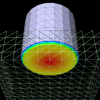
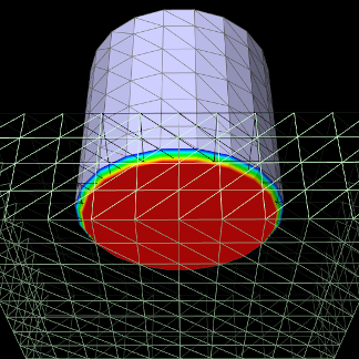
|
The model’s code is similar to that for ElasticFoundationContact (Section 8.7.4), except that the collidables are different and the EFC thickness property is bound to a field. The source code for the first part of the build method is shown below:
First, the cylinder and the plate are created as rigid bodies (lines 6-23), with the cylinder defined by a mesh read from the file data/beveledCylinder.obj relative to the demo source directory. The plate is fixed in place and positioned so that it is directly under the cylinder.
Next, the contact method is set to VERTEX_PENETRATION (as
required for EFC), this time by setting it for all collisions in the
collision manager, and a LinearElasticContact is constructed,
with ![]() ,
, ![]() , damping factor
, damping factor ![]() , and thickness
, and thickness ![]() (lines 25-32). Then in lines 34-43, a ScalarMeshField is created
for the cylinder surface mesh, with vertex values set so that the
field defines a thickness value
(lines 25-32). Then in lines 34-43, a ScalarMeshField is created
for the cylinder surface mesh, with vertex values set so that the
field defines a thickness value ![]() that increases with the radial
distance
that increases with the radial
distance ![]() from the cylinder axis according to:
from the cylinder axis according to:
This field is then added to the fields list of the MechModel and the EFC thickness property is bound to it (lines 44-46).
Lastly, a collision behavior is created, with the EFC added to it as a force behavior, and used to enable cylinder/plate collisions (lines 48-53).
It is important that EFC properties are bound to fields before the behavior method setForceBehavior() is called, because that method copies the force behavior and so subsequent field bindings would not be noticed. If for some reason the bindings must be made after the call, they should be applied to the copied force behavior, which can be obtained using getForceBehavior().
To run this example in ArtiSynth, select All demos > tutorial > VariableElasticContact from the Models menu. Running the model will result in contact pressures seen in the left of Figure 8.19, with the pressures decreasing radially in response to the increasing thickness. With no field binding, the pressures are constant across the cylinder bottom (Figure 8.19, right).
8.8 Monitoring collisions
Sometimes, an application may wish to know details about the collision interactions between a specific collidable and one or more other collidables. These details may include items such as contact forces or the penetration regions between the opposing meshes. This section describes ways in which these details can be observed through the use of collision responses.
8.8.1 Collision responses
Applications can track collision information by creating CollisionResponse components for the collidables in question and adding them to the MechModel using setCollisionResponse():
An alternate version of setCollisionResponse() creates the response component internally and returns it:
During every simulation step, the MechModel will update its response components to reflect the current collision conditions between the associated collidables.
The first collidable specified for a collision response must be a specific collidable component, while the second may be either another collidable or a group of collidables represented by a Collidable.Group:
When a compound collidable is specified, the response component will collect collision information for all its subcollidables.
As as with collision behaviors, the same response cannot be added to an application twice:
The complete set of methods for managing collision responses are similar to those for behaviors,
where getCollisionResponse() and clearCollisionResponse() respectively return and clear response components that have been previously set using one of the setCollisionResponse() methods.
8.8.2 Available information
Information that can be obtained from a CollisionResponse component includes whether or not the collidable is in collision, the current contact points, forces and pressures acting on the vertices of the colliding meshes, and the underlying CollisionHandler objects that maintain the contact constraints between each colliding mesh. Much of the available information is similar to that which can be displayed using collision rendering (Section 8.5).
The information methods provided by CollisionResponse are listed below. Many take a cidx argument to request information for either the first or second collidable, which refer, respectively, to the collidables specified by the arguments collidable0 and collidable1 in the setCollisionResponse() methods.
-
•
boolean inContact()
Queries if the collidables associated with the response are in contact. Note that this may be true even if the method getContactData() returns an empty list; this can occur, for instance, for vertex penetration contact when the collision meshes intersect in a small region without any interpenetrating vertices.
-
•
List<ContactData> getContactData()
Returns a list of the most recently computed contacts between the collidables. Each contact is described by a ContactData object supplying information about the contact points on each collidable, the normal, and contact and friction forces. If there are no current contacts, the returned list is empty. For more details on this information, consult the API documentation for ContactData and ContactPoint.
-
•
Map<Vertex3d,Vector3d> getContactForces(int cidx)
Returns a map of the contact forces acting on the vertices of the collision meshes of either the first or second collidable, as specified by setting cidx to 0 or 1. This information is most useful and accurate when using vertex penetration contact (Section 8.4.1.2).
-
•
Map<Vertex3d,Double> getContactPressures(int cidx)
Returns a map of the contact pressures acting on the vertices of the collision meshes of either the first or second collidable, as specified by setting cidx to 0 or 1. This information is most useful and accurate when using vertex penetration contact (Section 8.4.1.2).
-
•
ArrayList<PenetrationRegion> getPenetrationRegions(int cidx)
Returns a list of all the penetration regions on either the first or second collidable, as specified by setting cidx to 0 or 1. Penetration regions are available only if the collision manager’s collider type is set to AJL_CONTOUR (Section 8.4.2).
-
•
ArrayList<CollisionHandler> getHandlers()
Returns the CollisionHandlers for all currently active collisions associated with the collidables of the response.
A typical usage scenario for collision responses is to create them before the simulation is run, possibly in the root model build() method, and then query them when the simulation is running, such from the apply() method of a Monitor (Section 5.3). For example, in the root model build() method, the response could be created with the call
and then used in some runtime code as follows:
If for some reason it is difficult to store a reference to the response between its construction and its use, thengetCollisionResponse() can be used to retrieve it:
As with contact rendering, the information returned by a collision response may sometimes appear to lag the simulation by one time step. That is because contacts are computed at the end of each time step
8.8.3 Example: monitoring contact forces
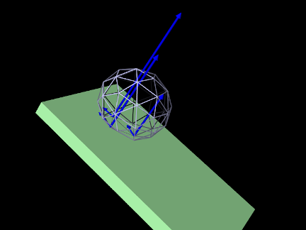
A simple example of using a CollisionResponse is given by
artisynth.demos.tutorial.ContactForceMonitor
This shows an FEM model of a ball rolling down an inclined plane, with a collision response combined with a Monitor used to print out the contact positions and forces at each time step. Contact forces are also rendered in the viewer. The model’s source code, excluding import statements, is shown below:
The build method creates a simple FEM ball and inclined plane, and positions the ball to an appropriate drop position (lines 27-42). The collisions are enabled between the ball and the plate, along with a CollisionResponse that is stored in the global reference myResp to allow it to be accessed from the monitor (lines 47-48).
The monitor itself is implemented by the class ContactMonitor, which is created by subclassing MonitorBase and overriding the apply() method to print out the contact information (lines 5-21). It does this by using the response’s getContactData() method to obtain a list of the contacts, and if there are any, printing the number of contacts, the time step start time (t0), and the position and force of each contact. An instance of the monitor is created and added to the root model at line 51.
Rendering is set so that the collision manager renders both the contact and friction forces in the viewer (lines 55-60), using blue arrows with a radius of 0.02 (line 60) and a scale factor for the arrow length of 0.0001 (line 58). To make the ball easy to see through, its elements are made invisible, and it is instead rendered using only its surface mesh, with face rendering disabled and edges drawn with a width of 2 (lines 63-67).
To run this example in ArtiSynth, select All demos > tutorial > ContactForceMonitor from the Models menu. Running the model will result in the ball colliding with the plane, showing the contact and friction forces as blue arrows (Figure 8.20), while the monitor prints out the contact positions and forces to the console at each time step, producing output like this:
8.8.4 Example: forces and pressures on mesh vertices
In the case of vertex penetration contact, contact forces are generated on the mesh vertices of both collidables in the vicinity of the intersection (Section 8.4.1.2 and Figure 8.11). The CollisionResponse methods getContactForces() and getContactPressures() can be used to obtain these forces, and their associated pressures, for the meshes of either the first or second collidable (corresponding to collidable0 or collidable1 in the setCollisionResponse() methods).
getContactForces() and getContactPressures() will also work for contour region contact (Section 8.4.1.1), but the results may be somewhat approximated and less meaningful.
As an example, the ContactForceMonitor in the example of Section 8.8.3 can be modified to find the maximum vertex contact force for a specific collidable by adding the following to the apply() method:
getContactForces() returns a map of the contact forces on each mesh vertex of the collidable indicated by collidableIdx (with 0 and 1 denoting the first and second collidables). To find the maximum force, one can simply iterate over the map. Similarly, maximum contact pressure can be determined using a code fragment like this:
Which collidable one chooses for evaluating contact forces or pressures will depend on the questions being asked by the modeling study. In the case of a FEM model colliding with a rigid body, one will almost certainly want to choose the FEM model as the collidable. In the case of two colliding FEMs (or two rigid bodies using vertex penetration contact), one may wish to use the collidable whose mesh has a higher resolution. While the forces and pressures on each collidable will be equal and opposite in aggregate, they will vary locally due to differences in the geometry and resolution of each collidable’s mesh. For instance, a collidable with a finer mesh will typically have a greater number of vertex forces of lesser magnitude.
8.9 Tips and limitations
This section describes practical tips that can employed when using ArtiSynth’s contact simulation, together with some of its limitations.
8.9.1 Contact jitter
ArtiSynth’s attempt to resolve the interpenetration of colliding bodies may sometimes cause a jittering behavior around the colliding area, as the surface collides, separates, and re-collides. This can usually be stabilized by maintaining a certain interpenetration distance during contact. This distance is controlled by the MechModel property penetrationTol. ArtiSynth attempts to compute a suitable default value for this property, but for some applications it may be necessary to control the value explicitly using the MechModel methods
8.9.2 Passing through objects
The ArtiSynth collision detection mechanism is static, which means that mesh intersections are computed at a fixed point in time and do not presently utilize velocity information. This means that if the colliding objects are fast enough or thin enough, it is possible for them to pass completely through each other during a simulation step (Figure 8.21, left). Similarly, even if objects do not pass completely through each other, the penetration may be large enough for contacts to be established with the wrong side (Figure 8.21, right).
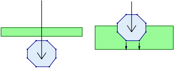
When this happens, there are two straightforward solutions:
-
1.
Reduce the simulation step size.
-
2.
Increase the thickness of one or more of the colliding meshes. This option is facilitated by the fact that, as mentioned in Section 8.3, collision meshes can be independent of a collidable’s physical geometry.
The problem of collidables passing through each other can be particularly acute in the case of shell elements, and consequently collisions involving shell elements are not fully supported. However, collisions involving shell elements will work in some circumstances, as described in Section 8.1.4.
8.9.3 Stray vertices
The stray vertex problem sometimes occurs when vertex penetration contact is used with objects with sharp edges. Because vertex penetration contacts are determined by finding the nearest face to each vertex on the opposing mesh, this may sometimes cause an inappropriate face to be selected if penetration is deep enough and near a sharp turn in the opposing mesh (Figure 8.22).
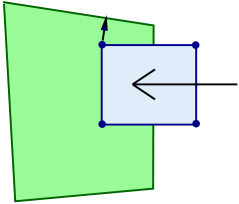
Possible solutions include:
-
1.
Reduce the simulation step size.
-
2.
Use the VERTEX_EDGE_PENETRATION contact method (Section 8.4.1.3).
-
3.
Adjust the mesh geometry or increase the mesh resolution; higher mesh resolutions will increase the number of contacts and reduce the impact of stray vertices.
8.9.4 Coulomb friction and stability
ArtiSynth uses a “box” friction approximation [10] to compute Coulomb (dry) friction, which allows for a less expensive and more robust computation at the expense of some accuracy. Box friction computes friction forces in two orthogonal directions in the plane perpendicular to the contact normal, using a fixed normal force taken from the previous solve, instead of employing the more detailed polyhedralized friction cones commonly used in multibody dynamics [1, 20]. The resulting linear complementarity problem is convex and hence more easily solved. Errors can be minimized by ensuring that one of the friction directions is parallel to the tangential contact velocity.
By default, friction forces are computed after the main velocity solve, in a secondary solve that does not use implicit integration techniques. This reduces compute time and works well for rigid bodies, or for FEM models when the friction forces are relatively small (which they often are in biomechanical applications). However, applications involving FEM models and large friction forces may suffer from instability. An example of this might be an FEM model resting on an inclined plane and relying on friction to remain stationary under a large load. To handle such situations, one can enable implicit friction integration by setting the useImplicitFriction property in MechModel; this can be done in code using the MechModel methods
At the time of this writing, implicit friction integration is a new ArtiSynth feature, and should be considered to be in beta testing.
When using implicit friction integration, if redundant contacts arise (typically between rigid bodies), it may be necessary to regularize both the contact constraints, using one of the methods described in Section 8.7, as well as the friction constraints, by setting the stictionCreep property of either the collision manager or behavior to a non-zero value, as described in Section 8.2.1.
Chapter 9 Muscle Wrapping and Via Points
ArtiSynth provides support for multipoint springs and muscles, which
are similar to axial springs and muscles (Sections
3.1.3 and 4.5), except that
they can contain multiple via points and also wrap around obstacles.
This allows the associated force directions to vary in response to
obstacles and constraints in the model, which is particularly
important in biomechanical models where point-to-point muscles need to
wrap around anatomical structures such as bones. A schematic
illustration is shown in Figure 9.1, where a
single spring connects points ![]() and
and ![]() , while passing through
a single via point
, while passing through
a single via point ![]() and wrapping around obstacles
and wrapping around obstacles ![]() and
and
![]() . Figure 9.2 shows two examples
involving a rigid body with fixed via points and a spring wrapping
around three rigid bodies.
. Figure 9.2 shows two examples
involving a rigid body with fixed via points and a spring wrapping
around three rigid bodies.
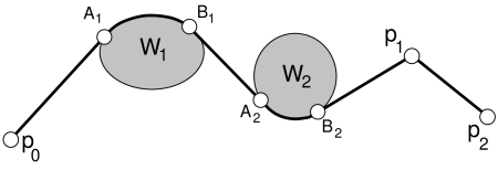
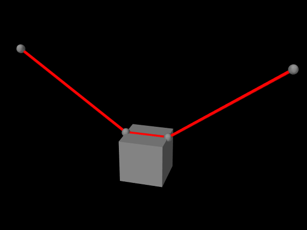 |
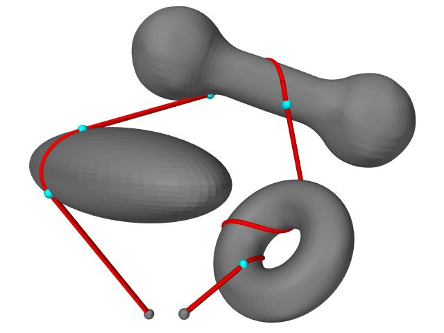 |
As with axial springs and muscles, multipoint springs and muscles must have two points to denote their beginning and end. In between, they can have any number of via points, which are fixed locations which the spring must pass through in the specified order. Any ArtiSynth Point object may be specified as a via point, including particles and markers. The purpose of the via point is generally to direct the spring along some particular path. In particular, the path directions before and after a via point will generally be different, and forces acting on the via point will be determined by the tension in the spring (or muscle) acting along these two different directions.
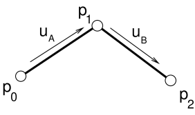
Conceptually, the spring or muscle “slides” through its via points, which act analogously to virtual three dimensional pulleys. In particular, the proportional distance between via points does not remain fixed.
The tension ![]() within the spring or muscle is computed from its
material, using the relation
within the spring or muscle is computed from its
material, using the relation ![]() described in Sections
3.1.3 and 4.5.1,
where
described in Sections
3.1.3 and 4.5.1,
where ![]() now denotes the entire length of the spring
as it passes through the via points and wraps around obstacles. The
total force
now denotes the entire length of the spring
as it passes through the via points and wraps around obstacles. The
total force ![]() acting on each via point is then given by
acting on each via point is then given by
where ![]() and
and ![]() are unit vectors giving the spring’s direction
immediately after and before the via point
(Figure 9.3).
are unit vectors giving the spring’s direction
immediately after and before the via point
(Figure 9.3).
Multipoint springs can also be made to wrap around one or more wrappable objects. Unlike via points, wrappable objects can occur in
any order along the spring and wrapping only occurs when the spring
and the object actually collide. Any ArtiSynth object that implements
Wrappable can be used as a wrapping object
(currently, only RigidBody objects
implement Wrappable).
The forces acting on a wrappable are those
generated by the forces ![]() and
and ![]() acting on the points
A and B where the spring makes and leaves contact with
it (Figure 9.4). These forces
are given by
acting on the points
A and B where the spring makes and leaves contact with
it (Figure 9.4). These forces
are given by
where ![]() and
and ![]() are unit vectors giving the spring’s direction
immediately before A and after B. Points A and B are collectively
known as the A/B points.
are unit vectors giving the spring’s direction
immediately before A and after B. Points A and B are collectively
known as the A/B points.
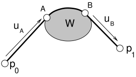
9.1 Via Points
Multipoint springs and muscles are implemented by the classes MultiPointSpring and MultiPointMuscle, respectively. The relationship between MultiPointSpring and MultiPointMuscle is the same as that between AxialSpring and Muscle: The latter is a subclass of the former, and allows the creation of active tension forces in response to its excitation property.
An application allocates one of these components, sets the appropriate material properties for the tension forces, and then adds points and wrappable objects as desired.
Points can be added, queried, and removed using the methods
| void addPoint (Point pnt) |
Add a point. |
| void addPoint (int idx, Point pnt) |
Add (insert) a point at index idx. |
| Point getPoint (int idx) |
Get the idx-th point. |
| int indexOfPoint (Point pnt) |
Returns the index of a point. |
| int numPoints() |
Return the number of points. |
| void setPoint (int idx, Point pnt) |
Replaces a point at index idx. |
| boolean removePoint (Point pnt) |
Remove a point. |
| void clearPoints () |
Removes all points. |
As with AxialSpring, there must be at least two points anchoring the beginning and end of the spring. Any additional points will be via points.
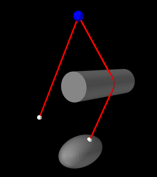 |
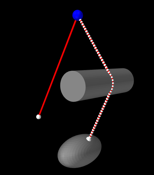 |
The section of a multipoint spring between any two adjacent points is known as a segment. By default, each segment forms a straight line between the two points and does not interact with any wrappable obstacles. To interact with wrappables, a segment needs to be declared wrappable, as described in Section 9.2.
Spring construction is illustrated by the following code fragment:
This creates a new MultiPointSpring and sets its material to a simple linear material with a specified stiffness and damping. Four points p0, p1, p2, p3 are then added, forming a start point, two via points, and a stop point.
9.1.1 Example: a muscle with via points
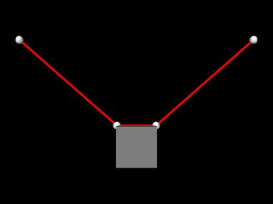
A simple example of a muscle containing via points is given by artisynth.demos.tutorial.ViaPointMuscle. It consists of a MultiPointMuscle passing through two via points attached to a block. The code is given below:
Lines 21-30 of the build() method create a MechModel and add a simple rigid body block to it. Two non-dynamic points (p0 and p1) are then created to act as muscle end points (lines 33-38), along with two markers (via0 and via1) which are attached to the block to act as via points (lines 41-44). The muscle itself is created by lines 42-53, with the end points and via points being added in order from start to end. The muscle material is a SimpleAxialMuscle, which computes tension according to the simple linear formula (4.1) described in Section 4.5.1. Lines 56-57 set render properties for the model, and line 59 creates a control panel (Section 5.1) that allows the muscle excitation property to be interactively controlled.
To run this example in ArtiSynth, select All demos > tutorial > ViaPointMuscle from the Models menu. The model should load and initially appear as in Figure 9.6. Running the model will cause the block to fall and swing about under gravity, while changing the muscle’s excitation in the control panel will vary its tension.
9.2 Obstacle Wrapping
As mentioned in Section 9.1, segments between pairs of via points can be declared wrappable, allowing them to interact with wrappable obstacles. This can be done as via points are added to the spring, using the methods
These make wrappable the next segment to be created (i.e., the segment
between the most recently added point and the next point to be added), with
numKnots specifying the number of knots that should be used to
implement the wrapping. Knots are points that divide the wrappable segment into
a piecewise linear curve, and are used to check for collisions with the
wrapping surfaces (Figure 9.5). If numKnots
is specified as ![]() , then the number of knots is computed automatically by
multiplying the initial length of the segment by the spring’s wrap knot
density returned by getWrapKnotDensity().
The argument initialPoints used by the second method is an optional
argument which, if non-null, can be used to specify initializing guide points
that give the segment an initial path around any obstacles (for more
details, see Section 9.4).
, then the number of knots is computed automatically by
multiplying the initial length of the segment by the spring’s wrap knot
density returned by getWrapKnotDensity().
The argument initialPoints used by the second method is an optional
argument which, if non-null, can be used to specify initializing guide points
that give the segment an initial path around any obstacles (for more
details, see Section 9.4).
Each wrappable segment will be capable of colliding with any of the wrappable obstacles that are known to the spring. Wrappables can be added, queried and removed using the following methods:
Unlike points, however, there is no implied ordering and wrappables can be added in any order and at any time during the spring’s construction.
Wrappable spring construction is illustrated by the following code fragment:
This creates a new MultiPointSpring with a linear material and three points p0, p1, and p2, forming a start point, via point, and stop point. The segment between p0 and p1 is set to be wrappable with 50 knot points. Two wrappable obstacles are added next, each of which will interact with the p0-p1 segment, but not with the non-wrappable p1-p2 segment. Finally, updateWrapSegments() is called to do an initial solve for the wrapping segments, so that they will be “pulled tight” around any obstacles before simulation begins.
It is also possible to make a segment wrappable after spring construction, using the method
where segIdx identifies the segment between points ![]() and
and
![]() . Several other methods can be used to modify or query the
number of knot points and/or initializing points after a segment has been
constructed:
. Several other methods can be used to modify or query the
number of knot points and/or initializing points after a segment has been
constructed:
| int getNumKnots (segIdx) |
Returns specified number of knots for segment segIdx. |
| int setNumKnots (int segIdx, int numKnots) |
Set specified number of knots for segment segIdx. |
| int numKnots (int segIdx) |
Returns actual number of knots for segment segIdx. |
| Point3d[] getInitializingPoints (int segIdx) |
Returns initializing points for segment segIdx. |
| void setInitializingPoints (int segIdx, Point3d[] initialPoints) |
Sets initializing points for segment segIdx. |
updateWrapSegments() should be called after any of the above set methods.
How many knots should be specified for a wrappable segment? Enough so
that the resulting piecewise-linear approximation to the wrapping
curve is sufficiently "smooth", and also enough to adequately detect
contact with the obstacles without passing through them. Values
between 50 and 100 generally give good results. Obstacles that are
small with respect to the segment length may necessitate more
knots. Making the number of knots very large will slow down the
computation (although the computational cost is only ![]() with
respect to the number of knots).
with
respect to the number of knots).
At the time of this writing, ArtiSynth implements two types of Wrappable object, both of which are instances of RigidBody. The first are specialized analytic subclasses of RigidBody, listed in Table 9.1, which define specific geometries and use analytic methods for the collision handling with the knot points. The use of analytic methods allows for greater accuracy and (possibly) computational efficiency, and so because of this, these special geometry wrappables should be used whenever possible.
| Wrappable | Description |
|---|---|
| RigidCylinder | A cylinder with a specified height and radius |
| RigidSphere | A sphere with a specified radius |
| RigidEllipsoid | An ellipsoid with specified semi-axis lengths |
| RigidTorus | A torus with specified inner and outer radii |
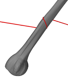 |
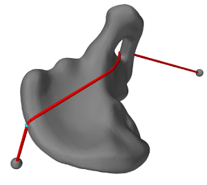 |
The second are general rigid bodies which are not analytic subclasses, and for which the wrapping surface is determined directly from the geometry of its collision mesh returned by getCollisionMesh(). (Typically the collision mesh corresponds to the surface mesh, but it is possible to specify alternates; see Section 3.2.9.) This is useful in that it permits wrapping around arbitrary mesh geometries (Figure 9.7), but in order for the wrapping to work well, these geometries should be smooth, without sharp edges or corners. Wrapping around general meshes is implemented using a quadratically interpolated signed-distance grid (Section 4.6), and the resolution of this grid also affects the effective smoothness of the wrapping surface. More details on this are given in Section 9.3.
9.2.1 Example: wrapping around a cylinder
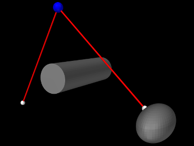
A example showing multipoint spring wrapping is given by artisynth.demos.tutorial.CylinderWrapping. It consists of a MultiPointSpring passing through a single via point, with both segments on either side of the point made wrappable. Two analytic wrappables are used: a fixed RigidCylinder, and a moving RigidEllipsoid attached to the end of the spring. The code, excluding import directives, is given below:
Lines 4-17 of the build() method create a MechModel with two fixed particles via0 and p1 to be used as via and stop points. Next, two analytic wrappables are created: a RigidCylinder and a RigidEllipsoid, with the former fixed in place and the latter connected to the start of the spring via the marker p0 (lines 20-37). Collisions are enabled between these two wrappables at line 40. The spring itself is created (lines 44-52), using setSegmentWrappable() to make the segments (p0, via0) and (via0, p1) wrappable with 50 knots each, and addWrappable() to make it aware of the two wrappables. Finally, render properties at set (lines 55-58), and a control panel (Section 5.1) is added that allows the spring’s drawKnots and drawABPoints properties to be interactively set.
To run this example in ArtiSynth, select All demos > tutorial > CylinderWrapping from the Models menu. The model should load and initially appear as in Figure 9.8. Running the model will cause the ellipsoid to fall and the spring to wrap around the cylinder. Using the pull tool (Section “Pull Manipulation” in the ArtiSynth User Interface Guide) on the ellipsoid can cause additional motions and make it also collide with the spring. Selecting drawKnots or drawABPoints in the control panel will cause the spring to render its knots and/or A/B points.
9.3 General Surfaces and Distance Grids
As mentioned in Section 9.2, wrapping around general mesh geometries is implemented using a quadratically interpolated signed distance grid. By default, for a rigid body, this grid is generated automatically from the body’s collision mesh (as returned by getCollisionMesh(); see Section 8.3).
Using a distance grid allows very efficient collision handling between the body and the wrap segment knots. However, it also means that the true wrapping surface is not actually the collision mesh itself, but instead the zero-valued isosurface associated with quadratic grid interpolation. Well-behaved wrapping behavior requires that this isosurface be smooth and free of sharp edges, so that knot motions remain relatively smooth as they move across it. Quadratic interpolation helps with this, which is the reason for employing it. Otherwise, one should try to ensure that (a) the collision mesh from which the grid is generated is itself smooth and free of sharp edges, and (b) the grid has sufficient resolution to not introduce discretization artifacts.
Muscle wrapping is often performed around structures such as bones, for which the representing surface mesh is often insufficiently smooth (especially if segmented from medical image data). In some cases, the distance grid’s quadratic interpolation may provide sufficient smoothing on its own; to determine this, one should examine the quadratic isosurface as described below. In other cases, it may be necessary to explicitly smooth the mesh itself, either externally or within ArtiSynth using the LaplacianSmoother class, which can apply iterations of either Laplacian or volume-preserving Taubin smoothing, via the method
Here numi is the number of iterations and lam and mu
are the Taubin parameters. Setting ![]() and
and ![]() results in traditional Laplacian smoothing. If this causes the mesh to
shrink more than desired, one can counter this by setting lam
and mu to values used for Taubin smoothing, as described in
[26].
results in traditional Laplacian smoothing. If this causes the mesh to
shrink more than desired, one can counter this by setting lam
and mu to values used for Taubin smoothing, as described in
[26].
If the mesh is large (i.e., has many vertices), then smoothing it may take noticeable computational time. In such cases, it is generally best to simply save and reuse the smoothed mesh.
By default, if a rigid body contains only one polygonal mesh, then its surface and collision meshes (returned by getSurfaceMesh() and getCollisionMesh(), respectively) are the same. However, if it is necessary to significantly smooth or modify the collision mesh, for wrapping or other purposes, it may be desirable to use different meshes for the surface and collision. This can be done by making the surface mesh non-collidable and adding an additional mesh that is collidable, as discussed in Section 3.2.9 as illustrated by the following code fragment:
Here, to ensure that the wrapping mesh does not contribute to the body’s inertia, its hasMass property is set to false.
Although it is possible to specify a collision mesh that is separate from the surface mesh, there is currently no way to specify separate collision meshes for wrapping and collision handling. If this is desired for some reason, then one alternative is to create a separate body for wrapping purposes, and then attach it to the main body, as described in Section 9.5.
To verify that the distance grid’s quadratic isosurface is sufficiently smooth for wrapping purposes, it is useful to visualize both the distance grid and its isosurface directly, and if necessary adjust the resolution used to generate the grid. This can be accomplished using the body’s DistanceGridComp, which is a subcomponent named distanceGrid and which may be obtained using the method
A DistanceGridComp exports a number of properties that can be used to control the grid’s visualization, resolution, and fit around the collision mesh. These properties are described in detail in Section 4.6, and can be set either in code using their set/get accessors, or interactively using custom control panels or by selecting the grid component in the GUI and choosing Edit properties ... from the right-click context menu.
When rendering the mesh isosurface, it is usually desirable to also disable rendering of the collision meshes within the rigid body. For convenience, this can be accomplished by setting the body’s gridSurfaceRendering property to true, which will cause the grid isosurface to be rendered instead of the body’s meshes. The isosurface type will be that indicated by the grid component’s surfaceType property (which should be QUADRATIC for the quadratic isosurface), and the rendering will occur independently of the visibility settings for the meshes or the grid component.
9.3.1 Example: wrapping around a bone
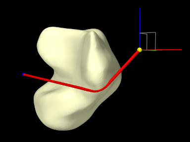 |
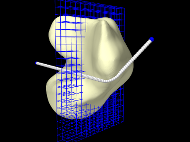 |
An example of wrapping around a general mesh is given by artisynth.demos.tutorial.TalusWrapping. It consists of a MultiPointSpring anchored by two via points and wrapped around a rigid body representing a talus bone. The code, with include directives omitted, is given below:
The mesh describing the talus bone is loaded from the file "data/TalusBone.obj" located beneath the model’s source directory (lines 11-19), with the utility class PathFinder used to determine the file path (Section 2.6). To ensure better wrapping behavior, the mesh is smoothed using Laplacian smoothing (line 21) before being used to create the rigid body (lines 23-27). The spring and its anchor points p0 and p1 are created between lines 30-49, with the talus added as a wrappable. The spring contains a single segment which is made wrappable using 100 knots, and initialized with an intermediate point (line 45) to ensure that it wraps around the bone in the correct way. Intermediate points are described in more detail in Section 9.4.
Render properties are set at lines 52-56; this includes turning off rendering for grid normals by zeroing the lineWidth render property for the grid component.
Finally, lines 59-67 create a control panel (Section 5.1) for interactively controlling a variety of properties, including gridSurfaceRendering for the talus (to see the grid isosurface instead of the bone mesh), resolution, maxResolution, renderGrid, and renderRanges for the grid component (to control its resolution and visibility), and drawKnots and wrapDamping for the spring (to make knots visible and to adjust the wrap damping as described in Section 9.6).
To run this example in ArtiSynth, select All demos > tutorial > TalusWrapping from the Models menu. Since all of the dynamic components are fixed, running the model will not cause any initial motion. However, while simulating, one can use the viewer’s graphical dragger fixtures (see the section “Transformer Tools” in the ArtiSynth User Interface Guide) to move p0 or p1 and hence pull the spring across the bone surface (Figure 9.9, left). One can also interactively adjust the property settings in the control panel to view the grid, isosurface, and knots, and the adjust the grid’s resolution. Figure 9.9, right, shows the model with renderGrid and drawKnots set to true and renderRanges set to "10:12 * *".
9.4 Initializing the Wrap Path
By default, when a multipoint spring or muscle is initialized (either at the start of the simulation or as a result of calling updateWrapSegments()), each wrappable segment is initialized to a straight line between its via points. This path is then adjusted to avoid and wrap around obstacles, using artificial linear forces as described in Section 9.6. The result is a local shortest path that wraps around obstacles instead of penetrating them. However, in some cases, the initial path may not be the one desired; instead, one may want it to wrap around obstacles some other way. This can be achieved by specifying additional intermediate points to initialize the segment as a piecewise linear path which threads its way around obstacles in the desired manner (Figure 9.10). These are specified using the optional initialPnts argument to the setSegmentWrappable() methods.
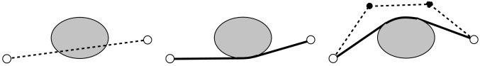
When initial points are specified, it is recommended to finish construction of the spring or muscle with a call to updateWrapSegments(). This fits the wrappable segments to their correct path around the obstacles, which can then be seen immediately when the model is first loaded. On the other hand, by omitting an initial call to updateWrapSegments(), it is possible to see the initial path as specified by the initial points. This may be useful to verify that they are in the correct locations.
MechModel also supplies a convenience method, updateWrapSegments()), which calls updateWrapSegments() for every multipoint spring contained within it.
In some cases, initial points may also be necessary to help ensure that the initial path does not penetrate obstacles. While obstacle penetration will normally be resolved by the artificial forces described in Section 9.6, this may not always work correctly if the starting path penetrates an obstacle too deeply.
9.4.1 Example: wrapping around a torus
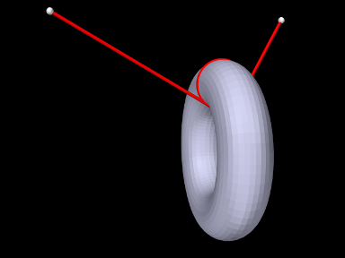
An example of using initial points is given by artisynth.demos.tutorial.TorusWrapping, in which a spring is wrapped completely around the inner section of a torus. The primary code for the build method is given below:
The mech model is created in the usual way with frame and rotary damping set to 1 and 10 (lines 4-5). The torus is created using the analytic wrappable RigidTorus (lines 8-14). The spring start and end points p0 and p1 are created at lines (17-22), and the spring itself is created at lines (26-41), with six initial points being specified to setSegmentWrappable() to wrap the spring completely around the torus inner section.
To run this example in ArtiSynth, select All demos > tutorial > TorusWrapping from the Models menu. The torus will slide along the wrapped spring until it reaches equilibrium.
9.5 Alternate Wrapping Surfaces
Although it common to use the general mesh geometry of a RigidBody as the wrapping surface, situations may arise where it is desirable to not do this. These may include:
-
•
The general mesh geometry is not sufficiently smooth to form a good wrapping surface;
-
•
Wrapping around the default mesh geometry is not stable, in that it is too easy for the wrap strand to “slip off”;
-
•
Using one of the simpler analytic geometries (Table 9.1) may result in a more efficient computation.
There are a couple of ways to handle this. One, discussed in Section 9.3, involves creating a collision mesh which is separate from the general mesh geometry. However, that same collision mesh must then also be used for collision handling (Chapter 8). If that is undesirable, or if multiple wrapping surfaces are needed, then a different approach may be used. This involves creating the desired wrappable as a separate object and then attaching it to the main RigidBody. Typically, this wrappable will be created with zero mass (or density), so that it does not alter the effective mass or inertia of the main body. The general procedure then becomes:
-
1.
Create the main RigidBody with whatever desired geometry and inertia is needed;
-
2.
Create the additional wrappable object(s), usually with zero density/mass;
-
3.
Attach the wrappables to the main body using one of the MechModel attachFrame() methods described in Section 3.9.3.
9.5.1 Example: wrapping for a finger joint
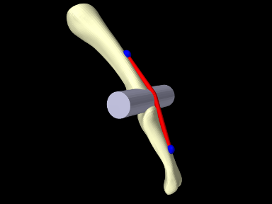
An example using an alternate wrapping surface is given by artisynth.demos.tutorial.PhalanxWrapping, which shows a muscle wrapping around a joint between two finger bones. Because the bones themselves are fairly narrow, using them as wrapping surfaces would likely lead to the muscle slipping off. Instead, a RigidCylinder is used for the wrapping and attached to one of the bones. The code, with include directives excluded, is given below:
The method createBody() (lines 6-14) creates a rigid body from a geometry mesh stored in a file in the directory “data” beneath the source directory, using the utility class PathFinder used to determine the file path (Section 2.6).
Within the build() method, a MechModel is created containing two rigid bodies representing the bones, proximal and distal, with proximal fixed and distal free to move with a frame damping of 0.03 (lines 18-28). A cylindrical joint is then added between the bones, along with markers describing the muscle’s origin and insertion points (lines 31-42). A RigidCylinder is created to act as a wrapping obstacle and attached to the distal bone in the same location as the joint (lines 46-50); since it is created with a density of 0 it has no mass and hence does not affect the bone’s inertia. The muscle itself is created at lines 53-64, using a SimpleAxialMuscle as a material and an extra initial point specified to setSegmentWrappable() to ensure that it wraps around the cylinder in the correct way (Section 9.4). Finally, some render properties are set at lines 67-69.
To run this example in ArtiSynth, select All demos > tutorial > PhalanxWrapping from the Models menu. The model should load and initially appear as in Figure 9.12. When running the model, one can move the distal bone either by using the pull tool (Section “Pull Manipulation” in the ArtiSynth User Interface Guide), or selecting the muscle in the GUI, invoking a property dialog by choosing Edit properties ... from the right-click context menu, and adjusting the excitation property.
9.5.2 Example: toy muscle arm with wrapping
|
|
A more complex example of wrapping, combined with multiple joints and point-to-point muscles, is given by artisynth.demos.tutorial.ToyMuscleArm, which depicts a two-link “arm”, connected by hinge joints, with opposing muscles controlling the poses of each link. The code, with import directives excluded, is given below:
Within the build() method, the mech model is created in the usual way and inertial damping is set to 1.0 (lines 73-75). Next, the rigid bodies depicting the base and links are created (lines 78-93). All bodies are created from meshes, with the base being made non-dynamic and the poses of the links set so that they line up vertically in their start position (Figure 9.13, left). A massless cylinder is created to provide a wrapping surface around the second hinge joint and attached to link1 (lines 96-109).
Hinge joints (Section 3.5.1) are then added between the base and link0 and link0 and link1 (lines 103-104), using the convenience method addHingeJoint() (lines 58-70). This method creates a hinge joint at a prescribed position in the x-z plane, uses it to connect two bodies, sets the range for the joint angle theta, and sets properties to render the shaft in blue.
Next, point-to-point muscles are placed on opposite sides of each link (lines 106-111). For link0, two Muscle components are used, added with the method addMuscle() (lines 18-29); this method creates a muscle connecting two bodies, using frame markers whose positions are specified in world coordinates in the x-z plane, and a SimpleMuscleMaterial (Section 4.5.1.1) with prescribed stiffness and maximum active force. For link1, MultiPointMuscle components are used instead so that they can be wrapped around the wrapping cylinder. These muscles are created with the method addWrappedMuscle() (lines 35-51), which creates a multipoint muscle connecting two bodies, using a single wrappable segment between two frame markers (also specified in the x-z plane). After the muscle is placed, its updateWrapSegments() method is called to “shrink wrap” it around the cylinder.
A marker is attached to the tip on link1 at lines 114-115, and then the links are repositioned, by setting the joint angles, so that the arm is not initially upright and will hence move when first run (lines 119-120). After repositioning, all wrap paths are updated by calling the MechModel method updateWrapSegments() (line 121), and the rest lengths for all muscles are set to their current lengths so that they will not initially exert passive tension (lines 124-127).
A control panel is created to allow runtime adjustment of the four muscle excitation values (lines 130-135), and render properties are set at lines 139-143.
9.6 Tuning the Wrapping Behavior
Wrappable segments are implemented internally using artificial linear elastic forces to draw the knots together and keep them from penetrating obstacles. These artificial forces are invisible to the simulation: the wrapping segment has no mass, and the knot forces are used to create what is essentially a first order physics that “shrink wraps” each segment around the obstacles at the beginning of each simulation step, forming a shortest-distance geodesic curve from which the wrapping contact points A and B are calculated. This process is now described in more detail.
Assume that a wrappable segment has ![]() knots, indexed by
knots, indexed by ![]() , each located at a position
, each located at a position ![]() . Two types of
artificial forces then act on each knot: a wrapping force
that pulls it closer to other knots, and contact forces that
push it away from wrappable obstacles. The wrapping force is given by
. Two types of
artificial forces then act on each knot: a wrapping force
that pulls it closer to other knots, and contact forces that
push it away from wrappable obstacles. The wrapping force is given by
where ![]() is the wrapping stiffness. To determine the contact
forces, we compute, for each wrappable, the knot’s distance to the
surface
is the wrapping stiffness. To determine the contact
forces, we compute, for each wrappable, the knot’s distance to the
surface ![]() and associated normal direction
and associated normal direction ![]() , where
, where ![]() implies that the knot is inside. These quantities are determined
either analytically (for analytic wrappables, Table
9.1), or using a signed distance grid (for
general wrappables, Section 9.3). The
contact forces are then given by
implies that the knot is inside. These quantities are determined
either analytically (for analytic wrappables, Table
9.1), or using a signed distance grid (for
general wrappables, Section 9.3). The
contact forces are then given by
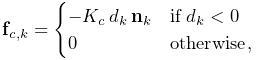 |
where ![]() is the contact stiffness.
is the contact stiffness.
The total force ![]() acting on each knot is then given by
acting on each knot is then given by
where the latter term is the sum of contact forces for all wrappables.
If we let ![]() and
and ![]() denote the aggregate position and force vectors
for all knots, then computing the wrap path involves finding the
equilibrium position such that
denote the aggregate position and force vectors
for all knots, then computing the wrap path involves finding the
equilibrium position such that ![]() . This is done at the
beginning of each simulation step, or whenever updateWrapSegments() is called, and
is achieved iteratively using Newton’s method.
If
. This is done at the
beginning of each simulation step, or whenever updateWrapSegments() is called, and
is achieved iteratively using Newton’s method.
If ![]() and
and ![]() denote the positions and forces at iteration
denote the positions and forces at iteration ![]() ,
and
,
and
denotes the local force derivative (or “stiffness”), then the basic Newton update is given by
In practice, to help deal with the nonlinearities associated with contact, we use a damped Newton update,
| (9.1) |
where ![]() is a constant wrap damping parameter, and
is a constant wrap damping parameter, and ![]() is
an adaptively computed step size adjustment. The computation of
(9.1) can be performed quickly, in
is
an adaptively computed step size adjustment. The computation of
(9.1) can be performed quickly, in ![]() time, since
time, since ![]() is a block-tridiagonal matrix, and the number of
iterations required is typically small (on the order of 10 or less),
particularly since the iterative procedure continues across simulation
steps and so
is a block-tridiagonal matrix, and the number of
iterations required is typically small (on the order of 10 or less),
particularly since the iterative procedure continues across simulation
steps and so ![]() does not need to be brought to
does not need to be brought to ![]() for any given
step. The maximum number of Newton iterations used for each
time step is
for any given
step. The maximum number of Newton iterations used for each
time step is ![]() .
.
Again, it is important to understand the artificial knot forces
described here are separate from the physical spring/muscle tension forces
discussed in Sections 3.1.3 and 4.5.1, and only facilitate the computation of each wrappable segment’s path around obstacles.
The default values for the wrapping parameters are ![]() ,
, ![]() ,
, ![]() , and
, and ![]() , and these often give
satisfactory results without the need for modification. However, in
some situations the default muscle wrapping may not perform adequately
and it is necessary to adjust these parameters. Problems may include:
, and these often give
satisfactory results without the need for modification. However, in
some situations the default muscle wrapping may not perform adequately
and it is necessary to adjust these parameters. Problems may include:
-
•
The wrapping path does not settle down and tends to “jump around”. Solutions include increasing the damping parameter
or
the maximum number of wrap iterations  . For general wrapping
surfaces (Section 9.3), one should also
ensure that the surface is sufficiently smooth.
. For general wrapping
surfaces (Section 9.3), one should also
ensure that the surface is sufficiently smooth. -
•
A wrapping surface is too thin and so the wrapping path “jumps through” it. Solutions include increasing the damping parameter
, increasing the number of knots in the segment, or
decreasing the simulation step size. An alternative approach is to use
an alternative wrapping surface
(Section 9.5) that is thicker and
better behaved.
Wrapping parameters are exported as properties of MultiPointSpring and MultiPointMuscle, and may be changed in code (using their set/get accessors), or interactively, either by exposing them through a control panel, or by selecting the spring/muscle in the GUI and choosing Edit properties ... from the right-click context menu. Property values include:
- wrapStiffness
-
Wrapping stiffness
 between knot points
(default value 1). Since the wrapping behavior is determined by the
damping to stiffness ratio, it is generally not necessary to
change this value.
between knot points
(default value 1). Since the wrapping behavior is determined by the
damping to stiffness ratio, it is generally not necessary to
change this value. - wrapDamping
-
Damping factor
(default
value 10). Increasing this value relative to results in wrap
path motions that are smoother and less likely to penetrate obstacles,
but which are also less dynamically responsive. Applications generally
work with damping values between 10 and 100 (assuming  ).
). - contactStiffness
-
Contact stiffness
 used to resolve obstacle
penetration (default value 10). It is generally not necessary
to change this value. Decreasing it will increase the distance that
knots are permitted to penetrate obstacles, which may result in
a slightly more stable contact behavior.
used to resolve obstacle
penetration (default value 10). It is generally not necessary
to change this value. Decreasing it will increase the distance that
knots are permitted to penetrate obstacles, which may result in
a slightly more stable contact behavior. - maxWrapIterations
-
Maximum number of Newton iterations
per time step (default value 10). If the wrapping
simulation exhibits instability, particularly with regard to obstacle
contact, increasing the number of iterations (to say 100) may help.
In addition, MultiPointSpring and MultiPointMuscle also export the following properties to control the rendering of knot and A/B points:
- drawKnots
-
If true, renders the knot points in each wrappable segment. This can be useful to visualize the knot density. Knots are rendered using the style, size, and color given by the pointStyle, pointRadius, pointSize, and pointColor values of the spring/muscle’s render properties.
- drawABPoints
-
If true, renders the A/B points. These are the first and last points of contact that a wrap segment makes with each wrappable, and correspond to the points where the spring/muscle’s tension acts on that wrappable (Section 9 and Figure 9.4). A/B points are rendered using the style and size given by the pointStyle, pointRadius (
 ) and pointSize values of the spring/muscle’s render
properties, and the color given by the ABPointColor property.
) and pointSize values of the spring/muscle’s render
properties, and the color given by the ABPointColor property.
Chapter 10 Inverse Simulation
10.1 Overview
ArtiSynth supports an inverse simulation capability that allows the computation of the excitation signals (for muscles and other actuators) needed to track target trajectories for a set of source components within the model (typically points or frames). This is achieved using a specialized controller component known as a TrackingController, defined in the package
artisynth.core.inverse
An application model creates the tracking controller and configures it with the source components, the exciter components needed to effect the tracking, and probes or controllers to specify the target trajectories. Then at each simulation time step the controller computes the excitations (i.e., signals to the exciter components) that allow the trajectories to be followed as closely as possible, in a manner conceptually similar to computed muscle control in OpenSim [7].
It is currently recommended to run inverse simulation with hybrid solving disabled. Hybrid solving combines direct and iterative solution techniques to speed up sparse matrix solves within ArtiSynth’s integrators. However, it can occasionally cause stability issues when used with inverse control. Hybrid solves can be disabled in several ways:
- 1.
By setting hybridSolvesEnabled to false under “Settings > Simulation ...” in the GUI; see “Simulation” under “Settings and Preferences” in the ArtiSynth User Interface Guide. This change can be made to persist across ArtiSynth restarts.
- 2.
By calling the static method setHybridSolvesEnabled() of MechSystemSolver in the model’s build() method:
MechSystemSolver.setHybridSolvesEnabled(false);
10.1.1 Tracking controller operation
Let ![]() ,
, ![]() and
and ![]() be composite vectors describing the positions,
velocities and forces of all the components in the application model, and let
be composite vectors describing the positions,
velocities and forces of all the components in the application model, and let
![]() be a vector of excitation signals for all the excitation components
available to the controller.
be a vector of excitation signals for all the excitation components
available to the controller. ![]() can be decomposed into
can be decomposed into
| (10.1) |
where ![]() are the passive forces corresponding to zero excitation, and
are the passive forces corresponding to zero excitation, and
![]() are the active forces. During simulation, the controller computes
values for
are the active forces. During simulation, the controller computes
values for ![]() to best track the target trajectories.
to best track the target trajectories.
In the case of motion tracking, let ![]() and
and ![]() be the subvectors of
be the subvectors of ![]() and
and
![]() containing the positions and velocities of the source components, and let
containing the positions and velocities of the source components, and let
![]() and
and ![]() be the corresponding target trajectories. At the beginning of
each time step, the controller compares the current source velocity state
be the corresponding target trajectories. At the beginning of
each time step, the controller compares the current source velocity state
![]() with the desired target state
with the desired target state ![]() and uses this to
determine a desired source velocity
and uses this to
determine a desired source velocity ![]() for the next time step;
this computation is done by the motion tracker (Figure
10.1, Section 10.1.2).
An excitation generator then computes
for the next time step;
this computation is done by the motion tracker (Figure
10.1, Section 10.1.2).
An excitation generator then computes ![]() in order to try and make
in order to try and make ![]() match
match ![]() (Section 10.1.3).
(Section 10.1.3).
The excitation generator accepts a desired velocity
instead of a desired acceleration because ArtiSynth’s physics engine computes velocity changes directly.
10.1.2 Motion tracking
As mentioned above, the motion tracker computes a desired source velocity
![]() for the next time step based on the current source state
for the next time step based on the current source state ![]() and
desired target state
and
desired target state ![]() . This can be done in two ways: chase control (the default), and PD control.
. This can be done in two ways: chase control (the default), and PD control.
10.1.2.1 Chase control
Chase control simply sets ![]() to
to ![]() , plus an additional velocity that
tries to reduce the position error
, plus an additional velocity that
tries to reduce the position error ![]() over a specified time interval
over a specified time interval
![]() , called the chase time:
, called the chase time:
| (10.2) |
In general, ![]() should be greater than or equal to the simulation step size
should be greater than or equal to the simulation step size
![]() . If it is greater, then
. If it is greater, then ![]() will tend to lag behind
will tend to lag behind ![]() , but this will
also reduce the potential for overshoot due to system
nonlinearities. Conversely, if
, but this will
also reduce the potential for overshoot due to system
nonlinearities. Conversely, if ![]() if less than
if less than ![]() , then
, then ![]() is much
more likely to overshoot. The default value of
is much
more likely to overshoot. The default value of ![]() is 0.01.
is 0.01.
10.1.2.2 PD control
PD control computes a desired source acceleration ![]() based on
based on
| (10.3) |
and then integrates this to determine ![]() :
:
| (10.4) |
where ![]() is the simulation step size. PD control offers a greater ability to
adjust the tracking behavior than chase control, but it is often necessary to
tune the gain parameters
is the simulation step size. PD control offers a greater ability to
adjust the tracking behavior than chase control, but it is often necessary to
tune the gain parameters ![]() and
and ![]() . One rule of thumb is to
set their initial values such that (10.2) and
(10.4) are equal, which leads to
. One rule of thumb is to
set their initial values such that (10.2) and
(10.4) are equal, which leads to
The default values for ![]() and
and ![]() are
are ![]() and
and ![]() , corresponding to
, corresponding to
![]() and
and ![]() both equaling
both equaling ![]() . Lowering the value of
. Lowering the value of ![]() will reduce
overshoot but increase tracking lag.
will reduce
overshoot but increase tracking lag.
PD control is enabled and adjusted by setting the usePDControl, Kp and Kd properties of the motion target term to true (Section 10.3.3).
10.1.3 Generating excitations using a quadratic program
Given ![]() , the excitation generator computes
, the excitation generator computes ![]() to try and ensure that the
velocity at the end of the subsequent time step,
to try and ensure that the
velocity at the end of the subsequent time step, ![]() , satisfies
, satisfies
| (10.5) |
This is accomplished using a quadratic program.
First, for a broad class of problems, ![]() is linearly related to
is linearly related to ![]() ,
so that (10.1) simplifies to
,
so that (10.1) simplifies to
| (10.6) |
where ![]() is an excitation response matrix. Given (10.6),
it is possible to show (section “Inverse modeling”
in [11]) that
is an excitation response matrix. Given (10.6),
it is possible to show (section “Inverse modeling”
in [11]) that
where ![]() is the velocity with zero excitations and
is the velocity with zero excitations and ![]() is a
motion excitation response matrix. To best follow the trajectory, we
can compute
is a
motion excitation response matrix. To best follow the trajectory, we
can compute ![]() to minimize the quadratic cost function
to minimize the quadratic cost function
| (10.7) |
If we add in the constraint that excitations lie in the range ![]() , the problem takes the form of a quadratic program (QP)
, the problem takes the form of a quadratic program (QP)
| (10.8) |
In order to prioritize some target terms over others,
![]() can be modified to include weights, according to
can be modified to include weights, according to
| (10.9) |
where ![]() is a diagonal weighting matrix.
To handle excitation redundancy, where the size of
is a diagonal weighting matrix.
To handle excitation redundancy, where the size of ![]() exceeds the
size of
exceeds the
size of ![]() , we can add a regularization term
, we can add a regularization term
![]() , where
, where ![]() is a diagonal weight matrix that
can be used to adjust the relative importance of specific excitations:
is a diagonal weight matrix that
can be used to adjust the relative importance of specific excitations:
| (10.10) |
The matrix
described here is the inverse of the matrix
presented in [11].
10.1.4 Force tracking
Other cost terms can be added to the tracking controller. For
instance, we can request a force trajectory ![]() for a selected set
of force effectors. As with motions, the forces of these effectors
for a selected set
of force effectors. As with motions, the forces of these effectors
![]() at the end of step
at the end of step ![]() are linearly related to
are linearly related to ![]() via
via
where ![]() is the force with zero excitations and
is the force with zero excitations and ![]() is
the force excitation response matrix. The force trajectory can
then be tracked by minimizing
is
the force excitation response matrix. The force trajectory can
then be tracked by minimizing
| (10.11) |
where ![]() is a diagonal weighting matrix.
When tracking force targets, the target force trajectory
is a diagonal weighting matrix.
When tracking force targets, the target force trajectory ![]() is fed
directly into the excitation generator (Figure 10.2); there
is no equivalent of the motion tracker.
is fed
directly into the excitation generator (Figure 10.2); there
is no equivalent of the motion tracker.
To balance the effect of different cost terms, each is associated with
a weight (e.g., ![]() ,
, ![]() , and
, and ![]() for the motion, force and
regularization terms), so that the QP takes a form such as
for the motion, force and
regularization terms), so that the QP takes a form such as
| (10.12) |
10.1.5 Incremental computation
In some cases, the system forces are not linear with respect to the excitations (i.e., equation (10.6) is not valid). One situation where this occurs is when equilibrium muscle models are used (Section 4.5.3).
When forces are not linear in ![]() , the force relationship can be linearized
and the quadratic program can be reformulated in terms of excitation changes
, the force relationship can be linearized
and the quadratic program can be reformulated in terms of excitation changes ![]() ; for example,
; for example,
| (10.13) |
where ![]() denotes the excitation values at the beginning of
the time step. Excitations are then updated
according to
denotes the excitation values at the beginning of
the time step. Excitations are then updated
according to
Incremental computation can be enabled, at the expense of slower computation, by setting the tracking controller property computeIncrementally to true (Section 10.3.2).
10.1.6 Setting up the tracking controller
Applications will generally set up a tracking controller using the following steps inside the application’s build() method:
-
1.
Create an instance of TrackingController and add it to the application using the root model’s addController() method.
-
2.
Configure the controller with the available excitation components using its addExciter(ex) and addExciter(weight,ex) methods.
-
3.
Configure the controller to track position or force trajectories for selected source components, which may include Point, Frame, or ForceEffector components. These are specified to the controller using methods such as addPointTarget(point), addFrameTarget(frame), and addForceEffectorTarget(forceEffector). These methods return a target object, which is allocated and maintained by the controller, and which is used for specifying the target positions or forces.
-
4.
Create input probes or controllers to specify the desired trajectories for the sources added in Step 3. Trajectories are specified by using probes or controllers to set the appropriate properties of the target objects returned by the addXXXTarget() methods. Likewise, output probes or monitors can be created to record the excitations and the tracked positions or forces of the sources.
-
5.
Add other cost terms as needed. These may include an L2 regularization term, added using the controller’s addL2RegularizationTerm() method. Regularization attempts to minimize the norm of the excitation values and is needed to resolve redundancy if the excitation set has more degrees of freedom than the target space.
For historical reasons, the target position and target velocity properties described in Section 5.3.1.1 are not used by the tracking controller for target components; therefore, probes controlling target positions and velocities should be bound to the position and velocity properties.
-
6.
Set controller configuration parameters.
10.1.7 Example: moving a point with multiple Muscles
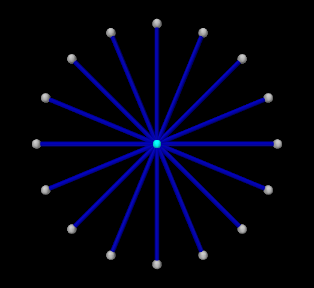 |
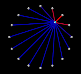 |
A simple example illustrating the steps of Section 10.1.6 is given by
artisynth.demos.tutorial.InverseParticle
which uses a set of point-to-point muscles to drive the position of a single particle. The model consists of a single dynamic particle, initially located at the origin, attached to a set of 16 point-to-point muscles arranged radially around it. A tracking controller is created to control the excitations of these muscles so as to enable the particle to follow a trajectory specified by a probe. The code for the model, without the package and import directives, is listed below:
The build() method begins by creating a MechModel in the usual way
and disabling gravity (lines 35-37). The particle to be controlled is then
created and placed at the origin and with a damping factor of 0.1 (lines
40-42). Next, the particle is attached to a set of point-to-point muscles that
are arranged radially around it (lines 45-48). These are created using the
method createMuscle() (lines 13-31), which attaches each to a fixed
non-dynamic particle located a distance of dist from the origin, and sets
its material to a SimpleAxialMuscle (Section 4.5.1.1)
with a passive stiffness, damping and maximum force (at excitation 1) defined
by muscleStiffness, muscleDamping, and muscleFmax (lines
4-6). Each muscle’s excitationColor and maxColoredExcitation
property is set so that its color transitions to red as its excitation value
varies from ![]() to
to ![]() (lines 28-29, Section 10.2.1.1),
and its rest length is initialized to its current length (line 30).
(lines 28-29, Section 10.2.1.1),
and its rest length is initialized to its current length (line 30).
After the model components have been built, a TrackingController is created and added to the root model’s controller set (lines 51-52). All of the muscles are then added to the controller as exciters to be controlled (lines 54-58). The particle is added to the controller as a motion source using the addPointTarget() method (line 60), which returns a target object in the form of a TargetPoint. Since the number of exciters exceeds the degrees-of-freedom of the target space, an L2-regularization term is added (line 63) to resolve the redundancy.
Rendering properties are set at lines 67-69: points in the model are rendered as gray spheres, except for the dynamic particle which is colored white, and the muscles are drawn as blue cylinders. (The target particle, which is contained within the controller, is displayed using its default color of cyan.)
Probes are created to specify the target trajectory and record the computed excitations. The first, targetprobe, is an input probe attached to the position property of the target component, running from time 0 to 1 (lines 72-79). Its data is specified in code using addData(), which specifies three knot points with a time step of 0.5. Interpolation is set to cubic (line 78) for greater smoothness. The second, exprobe, is a probe that records all the excitations computed by the controller (lines 82-85). It is created by the utility method createOutputProbe() supplied by the InverseManager class (Section 10.4.1).
To run this example, select All demos > tutorial > InverseParticle from the Models menu. The model should load and initially appear as in Figure 10.3 (left). When run, the controller computes excitations to move the particle along the trajectory specified by the probe, which is upward and to the right (Figure 10.3, right) and back again.
The target point created by the controller is rendered separately from the source point as a cyan-colored sphere (see Section 10.2.2.2). As the simulation proceeds and certain muscles are excited, their coloring changes from blue to red, in proportion to their excitation, in accordance with the properties excitationColor and maxColoredExcitation. Recorded data for both the trajectory and the computed excitation probes are shown in Figure 10.4.
10.2 Tracking controller components
This section describes in greater detail how exciters, motion and force sources, and other cost terms can be specified for the controller.
10.2.1 Exciters
An exciter can be any model component that implements
ExcitationComponent. These include
point-to-point Muscles (Section 4.5), muscle
bundles in FEM muscle models (Section 6.9.1.1), and MuscleExciters (Section 6.9.1.2). Each exciter exports an
excitation property which accepts a scalar input signal (usually in the
range ![]() ) that drives the exciter’s active force (or fans it out to other
exciters in the case of a MuscleExciter).
) that drives the exciter’s active force (or fans it out to other
exciters in the case of a MuscleExciter).
The set of excitation components used by a tracking controller is managed by the following methods:
| void addExciter(ExcitationComponent ex) |
Adds an exciter with default weight 1.0. |
| void addExciter(double w, ExcitationComponent ex) |
Adds an exciter with weight w. |
| void addExciters(Collection<ExcitationComponent> exciter) |
Adds a collection of exciters with weights 1.0. |
| int numExciters() |
Returns the number of exciters. |
| ExcitationComponent getExciter (int idx) |
Returns the idx-th exciter. |
| ListView<ExcitationComponent> getExciters() |
Returns a list of all exciters. |
| void clearExciters() |
Remove all exciters. |
An exciter’s weight forms its corresponding entry in the diagonal matrix ![]() used by the quadratic program ((10.10) and
(10.12)), with a smaller weight allowing the exciter to assume
greater prominence in the solution. Exciter weights can be managed with the
following methods:
used by the quadratic program ((10.10) and
(10.12)), with a smaller weight allowing the exciter to assume
greater prominence in the solution. Exciter weights can be managed with the
following methods:
| double getExcitationWeight (ExcitationComponent ex) |
Returns the weight for exciter ex. |
| void setExcitationWeight (ExcitationComponent ex, double w) |
Sets the weight for exciter ex. |
By default, the computed excitations are bounded by the interval ![]() , as
indicated in Section 10.1.3. However, these bounds can
be altered, either collectively using the tracking controller property excitationBounds, or individually for specific exciters:
, as
indicated in Section 10.1.3. However, these bounds can
be altered, either collectively using the tracking controller property excitationBounds, or individually for specific exciters:
| void setExcitationBounds(DoubleInterval range) |
Sets the excitationBounds property. |
| DoubleInterval getExcitationBounds() |
Queries the excitationBounds property. |
| void setExcitationBounds(ExcitationComponent ex, double low, double high) |
Sets excitation bounds for exciter ex. |
| DoubleInterval getExcitationBounds(ExcitationComponent ex) |
Queries excitation bounds for exciter ex. |
The excitation values themselves can also be queried and set with the following methods:
| void getExcitations(VectorNd values) |
Returns excitations in values. |
| double getExcitation(int idx) |
Returns the excitation of the idx-th exciter. |
By default, the controller initializes excitations to zero and then updates them at the beginning of each time step. However, when excitations are being computed incrementally (Section 10.1.5), it may be desirable to start with non-zero excitation values. In that case, the following methods may be useful:
| void initializeExcitations() |
Sets excitations to the current exciter values. |
| void setExcitations(VectorNd values) |
Sets excitations to values. |
The first sets the controller’s internal excitation values to those stored in the exciters, while the second sets both the internal values and the values in the exciters.
10.2.1.1 Excitation coloring
Some exciters (such as Muscle and MultiPointMuscle) support the ability to change color in proportion to their excitation value. This makes it easier to visualize the extent to which exciters are being activated within the model. Exciters which support this capability export the properties excitationColor, which is the color the exciter should transition to as excitation is increased, and maxColoredExcitation, which the excitation value at which the color transition is complete. In other words, the exciter’s color will vary from its default color to excitationColor as its excitation varies from 0 to maxColoredExcitation.
Excitation coloring does not occur if the exciter’s excitationColor is set to null.
The tracking controller exports a property, configExcitationColoring, which if true enables the automatic configuration of excitation coloring for exciters that support this capability. If enabled, then as these exciters are added to the controller, their excitationColor is inspected. If it has not been set (i.e., if it is null), then it is set to red and the nominal color for the exciter is set to white, enabling a white-to-red color transition for the exciter as it is activated.
10.2.2 Motion targets
As indicated above, motion source components can be specified to the controller using the addPointTarget() and addFrameTarget() methods. Source components may be instances of Point or Frame, and thereby may include both FEM nodes and rigid bodies. The methods for managing motion targets include:
| TargetPoint addPointTarget(Point source) |
Adds point source with weight 1.0. |
| TargetPoint addPointTarget(Point source, double w) |
Adds point source with weight w. |
| TargetFrame addFrameTarget(Frame source) |
Adds frame source with weight 1.0. |
| TargetFrame addFrameTarget(Frame source, double w) |
Adds frame source with weight w. |
| int numMotionTargets() |
Number of motion targets. |
| void removeMotionTarget(MotionTargetComponent source) |
Removes motion source. |
The addPointTarget() and addFrameTarget() methods each create and return a target component, allocated and contained within the controller, that mirrors the type of source component. These target components are either TargetPoint for point sources or TargetFrame for frame sources. Both TargetPoint and TargetFrame, together with the source components Point and Frame, are instances of MotionTargetComponent.
As simulation proceeds, the desired trajectory position ![]() for each source
component is specified by setting the target component’s position
property (or position, orientation and/or pose properties for
frame targets). As described elsewhere, this can be done using either probes
or other controller objects.
for each source
component is specified by setting the target component’s position
property (or position, orientation and/or pose properties for
frame targets). As described elsewhere, this can be done using either probes
or other controller objects.
For historical reasons, the target position and target velocity properties described in Section 5.3.1.1 are not used by the tracking controller for target components.
Likewise, a corresponding velocity trajectory ![]() can also be specified by
setting the velocity property of the target object. If this is not set,
can also be specified by
setting the velocity property of the target object. If this is not set,
![]() defaults to 0, which will introduce a small lag into the tracking
behavior. If
defaults to 0, which will introduce a small lag into the tracking
behavior. If ![]() is set, care should be taken to ensure that it is
consistent with the actual time derivative of
is set, care should be taken to ensure that it is
consistent with the actual time derivative of ![]() .
.
Applications typically do not need to specify
. However, doing so may improve tracking performance, particularly when using PD control (Section 10.1.2).
Each target component also implements the interface
TrackingTarget, described in
Section 10.2.8, which supplies methods to specify the
weights in the weighting matrix ![]() of the motion tracking cost term
of the motion tracking cost term
![]() (10.9).
(10.9).
Lists of all the motion source components and their associated target components (i.e., those returned by the addXXXTarget() methods) can be obtained using
| ArrayList<MotionTargetComponent> getMotionSources() |
Returns motion source components. |
| ArrayList<MotionTargetComponent> getMotionTargets() |
Returns motion target components. |
10.2.2.1 Motion target term
The cost term ![]() that is responsible for tracking motion targets is
contained within a tracking controller subcomponent that is named "motionTerm" and which is an instance of
MotionTargetTerm. Users
may access this component directly using
that is responsible for tracking motion targets is
contained within a tracking controller subcomponent that is named "motionTerm" and which is an instance of
MotionTargetTerm. Users
may access this component directly using
| MotionTargetTerm getMotionTargetTerm() |
Returns the controller’s motion target term. |
and then use it to set motion tracking properties such as those described in Section 10.3.3.
The motion tracking weight ![]() in (10.12) is
given by the weight property of the motion target term,
which can also be accessed directly by the controller methods
in (10.12) is
given by the weight property of the motion target term,
which can also be accessed directly by the controller methods
| double getMotionTargetTermWeight() |
Returns the motion target term weight. |
| void setMotionTargetTermWeight(double w) |
Sets the motion target term weight. |
10.2.2.2 Motion target rendering
The motion target components, which are allocated and maintained by the controller, are rendered by default, which makes it easy to visualize significant errors between the target positions and the tracked source positions. Target points are drawn as cyan colored spheres. For target frames, if the source component corresponds to a RigidBody, the target is rendered using a cyan colored wireframe copy of the source’s surface mesh.
Rendering of targets can be enabled or disabled by setting the tracking controller’s targetsVisible property. Otherwise, the application is free to set the render properties of individual target components, or their containing lists within the MotionTargetTerm, which can be accessed by the methods
| PointList<TargetPoint> getTargetPoints() |
Return all point motion target components. |
| RenderableComponentList<TargetFrame> getTargetFrames() |
Return all frame motion target components. |
Other methods of MotionTargetTerm allow the render properties for both the point and frame target lists to be set together:
| RenderProps getTargetRenderProps() |
Return render properties for the motion target lists. |
| void setTargetRenderProps (RenderProps props) |
Set render properties for the motion target lists. |
| void setTargetsPointRadius (double rad) |
Set pointRadius target render property to rad. |
10.2.3 Regularization
10.2.3.1 L2 Regularization
L2 regularization attempts to minimize the weighted square of the excitation values, as described by
| (10.14) |
in (10.12), and so provides a way to resolve redundancy when the number of exciters is greater than needed to perform the required tracking. It can be enabled or disabled by adding or removing an L2 regularization term from the controller, as managed by the following methods:
| void setL2Regularization() |
Enables L2 regularization with default weight 0.0001. |
| void setL2Regularization(double w) |
Enables L2 regularization with weight w. |
| double getL2RegularizationWeight() |
Returns regularization weight, or 0 if not enabled. |
| boolean removeL2Regularization() |
Removes L2 regularization. |
The weight associated with the above methods corresponds to ![]() in
(10.14) and (10.12). The entries in the
diagonal matrix
in
(10.14) and (10.12). The entries in the
diagonal matrix ![]() are given by the weights associated with the exciters
themselves, as described in Section 10.2.1.
are given by the weights associated with the exciters
themselves, as described in Section 10.2.1.
L2 regularization is implemented using a controller subcomponent of type L2RegularizationTerm, which is added or removed from the controller as required and can be accessed using
| L2RegularizationTerm getL2RegularizationTerm() |
Returns the controller’s L2 regularization term |
which will return null if regularization is not being applied.
Because the L2 regularizer tries to reduce the excitations ![]() , its use will
reduce the controller’s tracking accuracy. Therefore, the regularizer is often
employed with a weight value
, its use will
reduce the controller’s tracking accuracy. Therefore, the regularizer is often
employed with a weight value ![]() well below 1.0, with values around 0.1 or
0.01 being common. The best weight choice will of course depend on the
application.
well below 1.0, with values around 0.1 or
0.01 being common. The best weight choice will of course depend on the
application.
10.2.3.2 Excitation damping
The controller also provides a damping term that serves to minimize the time
derivative of ![]() , or more precisely,
, or more precisely,
where ![]() is the diagonal excitation weight matrix used for L2
regularization (10.14). Letting
is the diagonal excitation weight matrix used for L2
regularization (10.14). Letting ![]() denote
the excitations at the beginning of the time step, and approximating
denote
the excitations at the beginning of the time step, and approximating
![]() by
by
where ![]() is the time step size, the damping cost term
is the time step size, the damping cost term ![]() becomes
becomes
Excitation damping can be managed by the following methods:
| void setExcitationDamping() |
Enable excitation damping with default weight |
| void setExcitationDamping(double w) |
Enable excitation damping with weight w. |
| double getExcitationDampingWeight() |
Returns damping weight, or 0 if not enabled. |
| void removeExcitationDamping() |
Removes excitation damping. |
Excitation damping is implemented using a controller subcomponent of type DampingTerm, which is added or removed from the controller as required and can be accessed using
| DampingTerm getDampingTerm() |
Returns the controller’s excitation damping. |
which will return null if damping is not being applied.
10.2.4 Example: controlling ToyMuscleArm
A good tracking controller example is given by the model artisynth.demos.tutorial.InverseMuscleArm, which computes the muscle excitations needed to make the tip marker of the ToyMuscleArm demo (described in Section 9.5.2) follow a prescribed trajectory. The model extends artisynth.demos.tutorial.ToyMuscleArm, and then adds the tracking controller and probes needed to move the tip marker, as shown in the code below:
As mentioned above, this model extends ToyMuscleArm (line 1), and so calls super.build(args) in the build() method to create all the components of ToyMuscleArm. A tracking controller is then created (lines 7-8), and every Muscle and MultiPointMuscle is added to it as an exciter (lines 10-15).
Next, the marker at the tip of link1 (referenced by the inherited attribute myTipMkr) is added to the controller as a motion source (line 18) and the returned target object is stored in target. An L2 regularization term is added to the controller with weight 0.01 (line 20), and an input probe is created to provide the marker trajectory by setting the target’s position property (lines 22-37). The probe has a duration of 5 seconds, and the trajectory is a closed path, specified by 5 cubically interpolated knot points (line 36), that lie in the x-z plane and start at and return to the marker’s initial position x0, z0.
Probes are created to record the computed excitations and trace the desired and actual trajectories in the viewer. The first, exprobe, is created by the utility method createOutputProbe() supplied by the InverseManager class (lines 40-43, Section 10.4.1). The tracing probes are created by the RootModel method addTracingProbe() (lines 47-53), and two are created: one to trace the desired target by recording the position property of target, and another to trace the actual tracked (source) position by recording the position property of myTipMkr. The line colors of these are set to cyan and red, respectively, which specifies their display color in the viewer.
Lastly, an inverse control panel (Section 10.4.3) is created to manage controller properties (line 56), and some settings are made to allow for probe management by the InverseManager class, as discussed in Section 10.4.1 (lines 58-61); this includes setting the default probe duration to stopTime and the working folder to inverseMuscleArm located under the source folder.
To run this example, select All demos > tutorial > InverseMuscleArm from the Models menu. The model should load and initially appear as in Figure 10.5. When run, the controller will compute excitations to make the tip marker trace the desired trajectory, as shown in Figure 10.6 (left), where the tracing probe shows the target trajectory in cyan; the source trajectory appears beneath it in red but is largely invisible because it follows the target quite accurately. Computed excitation values are shown below. The target component created for the tip marker is rendered as a cyan-colored sphere (Section 10.2.2.2).
The muscles in InverseMuscleArm are initially colored white instead of red (as they are for ToyMuscleArm). That is because if a muscle’s excitationColor property is null, the controller automatically configures the muscle to vary in color from white to red as the muscle is activated, as described in Section 10.2.1.1. This behavior can be disabled by setting the controller property configExcitationColoring to false.
To illustrate how the L2 regularization weight can affect the tracking error, Figure 10.6 (right) shows the model run with a regularization weight of 10 instead of 0.1. The tracking error is now visible, with the red source trace probe clearly distinct from the cyan target trace. The computed muscle excitations are also noticeably different.
10.2.5 Example: controlling an FEM muscle model
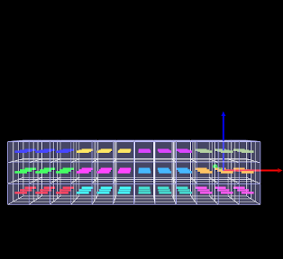
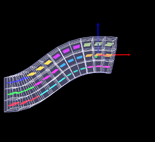
|
Another example involving an FEM muscle model is given by artisynth.demos.tutorial.InverseMuscleFem, which computes the muscle excitations needed to make an attached frame of the ToyMuscleFem demo (described in Section 6.9.4) follow a prescribed trajectory.
The model extends artisynth.demos.tutorial.ToyMuscleFem, and then adds the tracking controller and probes needed to move the tip marker, as shown in the code below:
Since the model extends ToyMuscleFem (line 1), the build() method begins by calling super.build(args) to create the model defined by the superclass. A tracking controller is then created and added to the root model’s controller set, all the muscle bundles in the FEM muscle model are added to it as exciters, and the attached frame is added to it as a motion source using addFrameTarget (lines 9-16).
An L2 regularization term is added, and then the motion tracking is set to use
PD control (Section 10.1.2), using gains of ![]() and
and ![]() (line 19-23).
(line 19-23).
To control position and orientation of the frame, two input probes are created (lines 27-38), one attached to the target’s position and the other to its orientation. (While it is possible to use a single probe to control both of these properties, or the single pose property, separate probes are used here to provide easier visualization.) Their data and settings are read from the probe files inverseFemFramePos.txt and inverseFemFrameRot.txt, located in the folder data beneath the application model source folder. Each specifies a probe in the time range from 0 to 5, with 26 knot points and cubic interpolation.
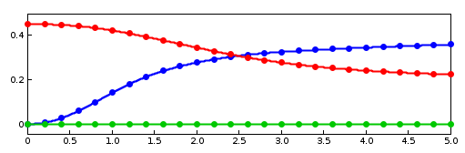 |
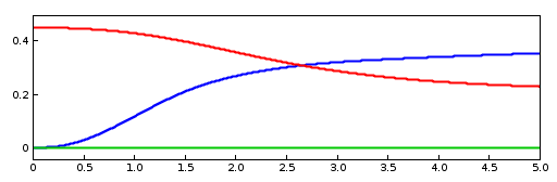 |
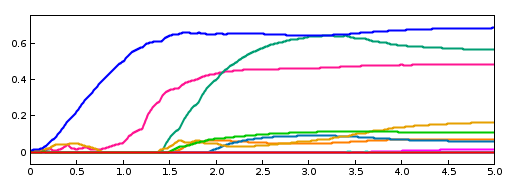 |
To monitor the controller’s tracking performance, two output probes are created and attached to the position and orientation properties of the source component myFrame (lines 58-67). Setting the interval argument to -1 in the probes’ constructors causes them to use the model’s current step size as the update interval. Finally, the utility class InverseManager (Section 10.4) is used to create an output probe for the computed excitations, as well as a control panel giving access to the various controller properties (lines 70-75).
To run this example, select All demos > tutorial > InverseMuscleFem from the Models menu. The model should load and initially appear as in Figure 10.7 (left). When run, the controller will compute excitations to move the attached frame along the specified position/orientation trajectory, reaching the final pose shown in Figure 10.7 (right). The target and actual source trajectories for the frame’s position (i.e., its origin) are shown in Figure 10.8, together with the computed excitations.
10.2.6 Force effector targets
The controller can also be asked to track a force trajectory for a set of force effector components; the excitations will then be computed to try to generate the prescribed forces. Any force component that implements the interface ForceTargetComponent can be used as a force effector source; this interface extends ForceEffector to supply several additional methods including:
At the time of this writing, ForceTargetComponents include:
| Component | Force size | Force description |
|---|---|---|
| AxialSpring | 1 | Tension in the spring |
| Muscle | 1 | Tension in the muscle |
| FrameSpring | 6 | Spring wrench as seen in body A (world coordinates) |
Controller methods for adding and managing force effector targets include:
| ForceEffectorTarget addForceEffectorTarget ( ForceTargetComponent source) |
Adds static-only force source with weight 1.0 |
| ForceEffectorTarget addForceEffectorTarget ( ForceTargetComponent source, double w) |
Adds static-only force source with weight w. |
| ForceEffectorTarget addForceEffectorTarget ( ForceTargetComponent source, double w, boolean staticOnly) |
Adds force source with weight w and static-only specified. |
| int numForceEffectorTargets() |
Number of force effector targets. |
| boolean removeForceEffectorTarget( ForceTargetComponent source) |
Removes force source. |
The addForceEffectorTarget() methods each create and return a
ForceEffectorTarget component.
As simulation proceeds, the desired target force for the source component is
specified by setting the target component’s targetForce property. As
described elsewhere, this can be done using either probes or other controller
objects. The target component also implements the interface
TrackingTarget, described in
Section 10.2.8, which supplies methods to specify the
weighting matrix ![]() in the force effector cost term
in the force effector cost term ![]() (10.11).
(10.11).
By default, force effector tracking is static-only, meaning that only static forces (i.e., forces that are not velocity dependent, such as damping) are considered. However, the third addForceEffectorTarget() method allows this to be explicitly specified.
Lists of all the force effector source components and their associated targets can be obtained using the methods:
| ArrayList<ForceEffectorTarget> getForceEffectorSources() |
Returns force effector source components. |
| ArrayList<ForceEffectorTarget> getForceEffectorTargets() |
Returns force effector target components. |
Specifying a force effector targetForce of 0 will have the same effect as minimizing the force associated with that force effector.
10.2.6.1 Force effector term
The cost term ![]() that is responsible for tracking force effector
targets is contained within a tracking controller subcomponent named
"forceEffectorTerm" and which is an instance of
ForceEffectorTerm.
This is added to the controller automatically whenever force effector tracking
is requested, and may accessed directly using
that is responsible for tracking force effector
targets is contained within a tracking controller subcomponent named
"forceEffectorTerm" and which is an instance of
ForceEffectorTerm.
This is added to the controller automatically whenever force effector tracking
is requested, and may accessed directly using
| ForceEffectorTerm getForceEffectorTerm() |
Returns the force effector term. |
The method will return null if the force effector term is not present.
The force effector tracking weight ![]() in (10.12) is
given by the weight property of the force effector term,
which can also be accessed directly by the controller methods
in (10.12) is
given by the weight property of the force effector term,
which can also be accessed directly by the controller methods
| double getForceEffectorTermWeight() |
Returns the force effector term weight. |
| void setForceEffectorTermWeight(double w) |
Sets the force effector term weight. |
10.2.7 Example: controlling tension in a spring
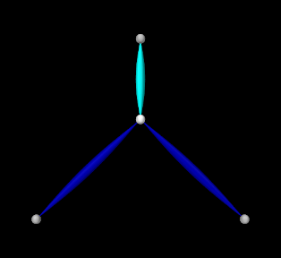 |
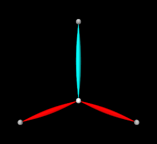 |
A simple example of force effector tracking is given by
artisynth.demos.tutorial.InverseSpringForce
which uses two point-to-point muscles to control the tension in a passive spring. The initial part of the code is the same as that for InverseParticle (Section 10.1.7), except for different parameter definitions,
which give the muscles different strengths and cause only 3 to be created
instead of 16, and the fact that the "center" particle is initially placed
at ![]() instead of the origin. The rest of the code diverges after
the tracking controller is created, as shown below:
instead of the origin. The rest of the code diverges after
the tracking controller is created, as shown below:
After the tracking controller is created (lines 18-19), the last two muscles are added to it as exciters (lines 21-23). The first muscle is then added as the force effector source using addForceEffectorTarget() (lines 26-28), which returns a target object. (The first muscle will be unactuated and so will behave as a passive spring.) Since the number of exciters exceeds the degrees-of-freedom of the target space, an L2-regularization term is added (line 31).
Rendering properties are set at lines 35-38: points are rendered as gray spheres, except for the center particle which is white, and muscles are drawn as spindles, with the exciter muscles blue and the passive target cyan.
Lastly, probes are created: an input probe to specify the target trajectory, an output probe to record target and tracked tensions, and an output probe to record the computed excitations. The first, targetprobe, is attached to the targetForce property of the target component and runs from time 0 to 1 (lines 41-48). Its data is specified in code using addData(), which specifies three knot points with a time step of 0.5. Interpolation is set to cubic (line 47) for greater smoothness. The second probe, trackingProbe, records both the target and source tension from the targetForce property of target and the forceNorm property of the passive spring (lines 52-61). The excitation probe is created by the utility method createOutputProbe() supplied by the InverseManager class (lines 64-67, Section 10.4).
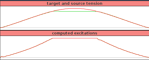
To run this example, select All demos > tutorial > InverseSpringForce from the Models menu. The model should load and initially appear as in Figure 10.9 (left). When run, the controller computes excitations to generate the requested tension in the passive spring; this causes the center particle to be pulled down (Figure 10.9, right). Both the target-source and computed excitation probes are shown in Figure 10.10.
For the middle third of the trajectory, the excitation values have reached their threshold value of 1 and so are unable to deliver more force. This in turn causes the source tension (green line) to deviate from the target tension (red line) in the target-source probe.
10.2.8 Target components
As described above, when a motion or force source is added to the controller
(using methods such as addPointTarget() or addForceEffectorTarget()), the controller creates and returns a target
component that is used for specifying the desired position or force
trajectory. Each target term also contains a scalar weight and a vector of
subweights, described by the properties weight and subWeights, all
of which have default values of 1.0. These weights are used to manage the
priority of the target within the tracking computation; the subWeights
vector has a size equal to the number of degrees of freedom (DOF) in the target
(3 for points and 6 for frames),
and permits fine-grained weighting for each of
the target’s DOFs. The product of the weight with each subweight produces the
entries for the diagonal weighting matrix that appears in the various cost
terms for motion and force tracking (e.g., ![]() for the motion tracking cost
function
for the motion tracking cost
function ![]() in (10.9) and
in (10.9) and ![]() for the force
effector cost function
for the force
effector cost function ![]() in (10.11)). Targets
(or specific DOFs) with higher weights will be tracked more accurately, while
weights of 0 effectively disable tracking.
in (10.11)). Targets
(or specific DOFs) with higher weights will be tracked more accurately, while
weights of 0 effectively disable tracking.
Target components vary depending on the source component whose position or force is being tracked, but each implements the interface TrackingTarget, which supplies the following methods for controlling the weights and subweights and querying the target’s source component:
| ModelComponent getSourceComp() |
Returns the target’s source component. |
|---|---|
| int getTargetSize() |
Returns number of target DOFs, which equals the number of subweights. |
| double getWeight() |
Returns the target component weight property. |
| void setWeight(double w) |
Sets the target component weight property. |
| Vector getSubWeights() |
Returns the target component subweights property. |
| void setSubWeights(VectorNd subw) |
Sets the target component subweights property. |
10.2.9 Point and frame exciters
In addition to muscle components, exciters may also include PointExciters and FrameExciters, which can be used to apply forces directly to Point or Frame components. This effectively gives the inverse controller the ability to do direct inverse simulation. These exciter components can also assume a role similar to that of the “reserve actuators” used in OpenSim [7], augmenting a model’s tracking capabilities to account for force sources that are not explicitly supplied by the model.
Each exciter applies a force along (or about) a single degree-of-freedom, as specified by the enumerated types PointExciter.ForceDof or FrameExciter.WrenchDof and described in the following table:
| Enum field | Description |
|---|---|
| ForceDof.FX | force along the point x axis |
| ForceDof.FY | force along the point y axis |
| ForceDof.FZ | force along the point z axis |
| WrenchDof.FX | force along the frame x axis (world coordinates) |
| WrenchDof.FY | force along the frame y axis (world coordinates) |
| WrenchDof.FZ | force along the frame z axis (world coordinates) |
| WrenchDof.MX | moment about the frame x axis (world coordinates) |
| WrenchDof.MY | moment about the frame y axis (world coordinates) |
| WrenchDof.MZ | moment about the frame z axis (world coordinates) |
Point or frame exciters may be created with the following constructors:
| PointExciter(Point point, FrameDof dof, double maxForce) |
Exciter for point with dof and maxForce. |
| PointExciter(String name, Point point, FrameDof dof, double maxForce) |
Named exciter for point with dof and maxForce. |
| FrameExciter(Frame frame, WrenchDof dof, double maxForce) |
Exciter for frame with dof and maxForce. |
| FrameExciter(String name, Frame frame, WrenchDof dof, double maxForce) |
Named exciter for frame with dof and maxForce. |
The maxForce argument specifies the maximum force (or moment) that the exciter supplies at an excitation value of 1.0.
If an exciter does not have sufficient strength to facilitate tracking, its excitation value is likely to saturate. This can often be solved by simply increasing the maxForce value.
To allow it to produce negative forces or moments along/about its specified
degree of freedom, the excitation bounds for a point or frame exciter
must be set to ![]() . The TrackingController does this
automatically whenever a point or frame exciter is added to it.
. The TrackingController does this
automatically whenever a point or frame exciter is added to it.
For convenience, PointExciter and FrameExciter provide static methods for creating sets of exciters to control all the translational forces and/or moments on a given point or frame:
| ArrayList<PointExciter> createPointExciters (MechModel mech, Point point, double maxForce, boolean createNames) |
Create three exciters to control all forces on a point. |
| ArrayList<FrameExciter> createFrameExciters ( MechModel mech, Frame frame, double maxForce, double maxMoment, boolean createNames) |
Create six exciters to control all forces and moments on a frame. |
| ArrayList<FrameExciter> createForceExciters (MechModel mech, Frame frame, double maxForce, boolean createNames) |
Create three exciters to control all forces on a frame. |
| ArrayList<FrameExciter> createMomentExciters ( MechModel mech, Frame frame, double maxMoment, boolean createNames) |
Create three exciters to control all moments on a frame. |
If the (optional) mech argument in these methods is non-null, the exciters are added to the MechModel’s forceEffectors list. If the argument createNames is true, and the point or frame itself has a non-null name, then the exciter is assigned a name based on the point/frame name and the degree of freedom.
10.2.10 Example: controlling ToyMuscleArm with FrameExciters
The InverseMuscleArm example of Section 10.2.4 can be modified to use frame exciters in place of its muscles, allowing link forces to be controlled directly to make the marker follow the specified path. The modified model is artisynth.demos.tutorial.InverseFrameExciterArm, and the sections of code where it differs from InverseMuscleArm are listed below:
After the controller is created (lines 43-44), four frame exciters are created to generate translational forces on each link in the x-z plane, up to a maximum force of 200 (lines 61-64). These exciters are created using the method addFrameExciter() (lines 32-37), which creates the exciter and adds it to the MechModel and to the controller’s exciter list.
Instead of calling the method addFrameExciter(), the frame exciters could have been generated using the following code fragment:
This would create six exciters instead of four (three forces per link, instead of limiting forces to x-z plane), but the additional forces would simply not be recruited by the controller.
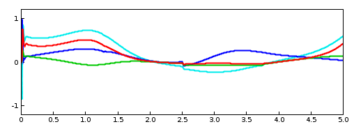
To run this example, select All demos > tutorial > InverseFrameExciterArm from the Models menu. The excitations generated by running the model are shown in Figure 10.11.
10.3 Tracking controller structure and settings
10.3.1 Controller structure
The tracking controller is a composite component, which contains the exciter list and the various cost and constraint terms as subcomponents. Some of these components are added as needed. They include the following, as described by their names:
- exciters
-
A list of references to the exciters which have been added to the controller. Note that this is a list of references; the exciters themselves exist elsewhere in the model. Always present.
- motionTerm
-
The MotionTargetTerm detailed in Section 10.2.2.1. Implements the motion cost term
 defined in
(10.7), and the motion tracker of
Figure 10.1. Allocates and maintains target components
for motion sources, storing the targets in the subcomponent lists targetPoints and targetFrames, and references to the sources in the
reference lists sourcePoints and sourceFrames. Always present.
defined in
(10.7), and the motion tracker of
Figure 10.1. Allocates and maintains target components
for motion sources, storing the targets in the subcomponent lists targetPoints and targetFrames, and references to the sources in the
reference lists sourcePoints and sourceFrames. Always present. - forceEffectorTerm
-
- boundsTerm
-
Implements the actuator bounds
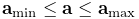 ,
where
,
where  and
and  are nominally
  and
and  . Always present.
 - L2RegularizationTerm
-
Implements the cost term for L2 regularization (Section 10.2.3.1). Added on demand.
- dampingTerm
-
Implements the cost term for excitation damping (Section 10.2.3.2). Added on demand.
10.3.2 Controller properties
The controller and its cost terms have a number of properties that can be used to adjust the controller’s behavior. They can be set interactively, either through the inverse controller panel created by the InverseManager (Section 10.4.3), or by selecting the relevant component in the navigation panel and choosing "Edit properties ..." from the context menu. The properties can also be set in code, using the accessor methods supplied by their host component. These methods will usually be named getXxx() and setXxx() for property xxx. Properties of the tracking controller itself include:
- active
-
Controls whether or not the controller is active. Setting this to false turns the controller off. Default value is true.
- normalizeCostTerms
-
Controls whether or not the cost terms are normalized. Normalizing the terms helps ensure that their weights (e.g.,
 ,
,  , and
, and  in
(10.12)) more accurately control the tradeoffs between terms.
Default value is true.
in
(10.12)) more accurately control the tradeoffs between terms.
Default value is true. - computeIncrementally
-
Controls whether excitation values should be computed incrementally, as described in Section 10.1.5. Default value is false.
- excitationBounds
-
Specifies the default excitation bounds for exciter components. Default value is
. - targetsVisible
-
Controls the visibility of the motion target terms contained within the controller, as described in Section 10.2.2.2. Default value is true.
- configExcitationColoring
-
If enabled, automatically configures exciters which support excitation coloring to vary from white to red as their excitation increases (Section 10.2.1.1). Default value is true.
- probeDuration
-
Default duration of probes managed by the InverseManager class (Section 10.4). Default value is 1.0.
- probeUpdateInterval
-
Default update interval of output probes managed by the InverseManager class (Section 10.4). Default value is -1, which means that the interval will default to the simulation step size.
- useKKTFactorization
-
Uses a more computationally expensive but possibly more accurate method to compute the excitation response matrices such as
 and
and  (Section 10.1.3). Default value is false.
 - maxExcitationJump
-
Experimental property that limits the change in excitation during any time step. Default value is false.
- useTimestepScaling
-
Experimental property which enables scaling of all the cost terms by the simulation time step. Default value is false.
- debug
-
Enables debugging messages. Default value is false.
10.3.3 Motion term properties
The motion target term (Section 10.2.2.1) exports a number of properties that control motion tracking:
- enabled
-
Controls whether or not this term is enabled. Default value is true.
- weight
-
Specifies the weight
of this term relative to the other cost
terms. Default value is 1.0. - chaseTime
-
Specifies the chase time
 used for chase control
(Section 10.1.2.1). Default value is 0.01.
used for chase control
(Section 10.1.2.1). Default value is 0.01. - usePDControl
-
Controls whether or not PD control is used (Section 10.1.2.2). Default value is false.
- Kp
-
Specifies the proportional terms for PD control (Section 10.1.2.2). Default value is 10000.
- Kd
-
Specifies the derivative terms for PD control (Section 10.1.2.2). Default value is 100.
- legacyControl
-
Controls whether or not legacy control is used. Default value is false.
10.3.4 Properties for other cost terms
All other cost terms, including the L2 regularization (Section 10.2.3.1), export the following properties:
- enabled
-
Controls whether or not the term is enabled. Default value is true.
- weight
-
Specifies the weight of this term relative to the other cost terms. Default value is 1.0.
10.4 Managing probes and control panels
The tracking controller package provides the helper class InverseManager to aid with the creation of probes and control panels that are useful in for inverse simulation applications. The functionality provided by InverseManager is described in this section, and additional documentation may be found in its API documentation.
10.4.1 Inverse simulation probes
| ProbeID | I/O type | Probe name | Default filename |
|---|---|---|---|
| TARGET_POSITIONS | input | "target positions" | target_positions.txt |
| INPUT_EXCITATIONS | input | "input excitations" | input_excitations.txt |
| TRACKED_POSITIONS | output | "tracked positions" | tracked_positions.txt |
| SOURCE_POSITIONS | output | "source positions" | source_positions.txt |
| COMPUTED_EXCITATIONS | output | "computed excitations" | computed_excitations.txt |
InverseManager contains static methods that support the creation and management of a variety of probes related to inverse simulation. These probes are defined by the enumerated type InverseManager.ProbeID, which includes the following identifiers:
- TARGET_POSITIONS
-
A PositionInputProbe (Section 5.4.8) which provides a trajectory
 for all motion targets. Its input values
are attached to the position property of each point target and the position and orientation properties of each frame target, in the order
the targets appear in the controller. The rotation representation is given by
the positionProbeRotRep property of the controller.
for all motion targets. Its input values
are attached to the position property of each point target and the position and orientation properties of each frame target, in the order
the targets appear in the controller. The rotation representation is given by
the positionProbeRotRep property of the controller. - INPUT_EXCITATIONS
-
An input probe which provides input excitation values for all the controller’s exciters, in the order they appear in the controller. This probe can be used for testing purposes, in order to see what trajectory can be expected to arise from a given excitation input.
- TRACKED_POSITIONS
-
A PositionOutputProbe which records the positions of all motion targets as they are set by the controller. Its output values are extracted from the same component properties used by TARGET_POSITIONS, and its rotation representation is given by the positionProbeRotRep property of the controller.
- SOURCE_POSITIONS
-
A PositionOutputProbe which records the actual position trajectory
 followed by all motion sources. Its output values are
extracted from the same component properties used by TARGET_POSITIONS,
and its rotation representation is given by the positionProbeRotRep
property of the controller.
followed by all motion sources. Its output values are
extracted from the same component properties used by TARGET_POSITIONS,
and its rotation representation is given by the positionProbeRotRep
property of the controller. - COMPUTED_EXCITATIONS
-
An output probe which records the computed excitation values for all the controller’s exciters, in the order they appear in the controller.
Each of these probes is associated with both a name and a default file name (Table 10.1), where the default file name may be assigned if another file path is not explicitly specified.
When a default file name is used, it is assumed to be relative to the ArtiSynth working folder, as described in Section 5.4.
These probes may be created, for a given tracking controller, with the following (static) InverseManager methods:
| NumericInputProbe createInputProbe (TrackingController tcon, ProbeID pid, String filePath, double start, double stop) |
Create input probe specified by pid. |
| NumericOutputProbe createOutputProbe (TrackingController tcon, ProbeID pid, String filePath, double start, double stop, double interval) |
Create output probe specified by pid. |
Here pid specifies the probe type, filePath an (optional) file path, start and stop the start and stop times, and interval the output probe update interval.
Created probes may be added to the application root model as needed.
Most of the examples above use createOutputProbe() to create a computed excitations probe. In InverseMuscleFem (Section 10.2.5), the two output probes used to display the tracked position and orientation of myFrame, created at lines (42-51), could be replaced by a single probe of type SOURCE_POSITIONS, using a code fragment like this:
Likewise, a probe showing the target position and orientation, for purposes of comparing it against SOURCE_POSITIONS and evaluating the tracking error, could be created using
For both these method calls, the source and target components (myFrame and target in the example) are automatically located within the tracking controller.
If the created probe is a PositionInputProbe or PositionOutputProbe, and one needs access to the features of that type, a cast will be necessary, e.g.:
One reason to create a TRACKED_POSITIONS probe, instead of comparing SOURCE_POSITIONS directly against the trajectory input probe, is that the former is guaranteed to have the same number of data points as SOURCE_POSITIONS, whereas a trajectory probe, being an input probe, may not. Moreover, if the trajectory is being produced using a controller, a trajectory probe may not even exist.
For convenience, InverseManager also provides methods to add a complete set of default probes to the root model:
| void addProbes (RootModel root, TrackingController tcon, double duration, double interval) |
Add default probes to root. |
| void resetProbes (RootModel root, TrackingController tcon, double duration, double interval) |
Clear probes and add default probes to root. |
addProbes() creates a COMPUTED_EXCITATIONS probe and an INPUT_EXCITATIONS probe, with the latter deactivated by default. If the controller has any motion targets, it will also create TARGET_POSITIONS, TRACKED_POSITIONS and SOURCE_POSITIONS probes. Probe start times are set to 0, stop times are set to duration, and the output probe update interval is set to interval, with -1 causing the interval to default to the simulation step size. Probe file names are set to the default file names described in Table 10.1. Since these file names are relative, the files themselves are assumed to exist in the ArtiSynth working folder, as described in Section 5.4. If the file for an input probe actually exists, it is used to initialize the probe’s data; otherwise, the probe data is initialized to 0 and the probe is deactivated.
resetProbes() removes all existing probes and then behaves identically to addProbes().
InverseManager also supplies methods to locate and adjust the probes that it has created:
| NumericInputProbe findInputProbe ( RootModel root, ProbeID pid) |
Find specified input probe. |
| PositionInputProbe findPositionInputProbe ( RootModel root, ProbeID pid) |
Find input probe, restricted to PositionInputProbes. |
| NumericOutputProbe findOutputProbe ( RootModel root, ProbeID pid) |
Find specified output probe. |
| PositionOutputProbe findPositionOutputProbe ( RootModel root, ProbeID pid) |
Find output probe, restricted to PositionOutputProbes. |
| Probe findProbe (RootModel root, ProbeID pid) |
Find specified input or output probe. |
| boolean setInputProbeData (RootModel root, ProbeID pid, double[] data, double timeStep) |
Set input probe data. |
| boolean setProbeFileName (RootModel root, ProbeID pid, String filePath) |
Set probe file path. |
The findProbe() methods search for the probe specified by pid within a root model, using the probe’s file name (Table 10.1) as a search key. The method setInputProbeData() searches for a specified probe, and if it is found, sets its data using the probe’s setData(double[],double) method and returns true. Likewise, setProbeFileName() searches for a specified probe and sets its file path.
Since probes maintained by InverseManager use probe names as a search key, care should be taken to ensure that these names do not conflict with those of other application probes.
10.4.2 Example: using InverseManager probes
The example InverseMuscleArm (Section 10.2.4) has been configured for use with the InverseManager by setting its working folder to inverseMuscleArm located beneath its source folder. If instead of creating the target and output excitations probes (lines 34-52), addProbes() is simply called at the end of the build() method (after the working folder has been set), as in
then a set of probes will be created as shown in Figure 10.13. The tracing probes ("target tracing" and "source tracing") are still present, in addition to five default probes. TARGET_POSITIONS and INPUT_EXCITATIONS are expanded to show the data that has been automatically loaded from the files target_positions.txt and input_excitations.txt located in the working folder. By default, the former probe is enabled and the latter is disabled. If the model is run, inverse simulation will proceed as before.
After loading the probes, the application could disable the tracking controller and enable the input excitations:
This will cause the simulation to run “open loop” in response to the excitations. However, because the input excitations are slightly different than those that were computed by the controller, there is now a considerable tracking error (Figure 10.14, left).
After the open loop run, one can save the resulting SOURCE_POSITIONS probe, which will write the file "source_positions.txt'' into the working folder. This can then be used to generate a new target trajectory, by copying it to "target_positions.txt". If the model is reloaded, the new trajectory will now appear in the TARGET_POSITIONS probe (Figure 10.15). Deactivating the INPUT_EXCITATIONS probe and reactivating the tracking controller will cause this new trajectory to be tracked properly (Figure 10.14, right).
In ways such as this, the probes may be used to examine the behavior and performance of the tracking controller.
|
|
10.4.3 Inverse control panel
InverseManager also provide methods to create and manage an inverse control panel, which allows interactive editing of the properties of the tracking controller and its various cost terms, as described in Section 10.3. Applications can create an instance of this panel in their build() method, as the InverseMuscleArm example (Section 10.2.4) does at line 65:
The panel is automatically configured to display the properties of the cost terms with which the controller is currently configured. Figure 10.16 shows the panel for InverseMuscleArm.
The following methods are supplied by InverseManager to manage inverse control panels:
| ControlPanel createInversePanel (TrackingController tcon) |
Create inverse control panel for tcon. |
| ControlPanel addInversePanel (RootModel root, TrackingController tcon) |
Create and add inverse control panel to root. |
| ControlPanel findInversePanel (RootModel root) |
Find inverse control panel in root. |
At the top of the inverse panel are three buttons: "reset probes", "sync excitations", and "sync targets". The first uses InverseManager.resetProbes() to clear all probes and recreate the default probes, using the duration and update interval specified by the tracking controller properties probeDuration and probeUpdateInterval. The second button copies the contents of the COMPUTED_EXCITATIONS probe into the INPUT_EXCITATIONS probe. If this is done after excitations have been computed, then running the simulation again with the controller deactivated and INPUT_EXCITATIONS activated should produce an identical motion. The third button copies the contents of the SOURCE_POSITIONS probe into the TARGET_POSITIONS. This can be used to verify that a source trajectory created open loop with a prescribed set of input excitations can in fact be tracked by the controller.
The probe copy methods used by the “sync” buttons are also available to the application code:
| boolean syncTargetProbes (RootModel root) |
Copy SOURCE_POSITIONS into TARGET_POSITIONS. |
| boolean syncExcitationProbes (RootModel root) |
Copy COMPUTED_EXCITATIONS into INPUT_EXCITATIONS. |
10.5 Inverse kinematics
ArtiSynth supplies an inverse kinematic solver, IKSolver, that can be used to compute the configuration of an articulated structure of rigid bodies given the positions of markers attached to those bodies. A primary use of this solver is to transform a marker trajectory, which may not fit the model well due to noise or registration issues, into one that is kinematically feasible given the joint constraints on the bodies. This can be an important preconditioning step for inverse dynamic simulation, as the resulting excitations do not then need to expend effort on infeasible targets.
10.5.1 Inverse kinematics solver
An IKSolver is created with the following constructors:
| IKSolver (MechModel mech, Collection<? extends Marker> mkrs) | |
| IKSolver (MechModel mech, Collection<? extends Marker> mkrs, VectorNd weights) |
mech is the MechModel containing the bodies and constraints, mkrs is a list of markers, and weights is an optional set of marker weight values. If weights is not specified, markers are assumed to have a weight of 1. Each marker is assumed to be either a FrameMarker or GenericMarker that is attached to a RigidBody; other marker types will cause an exception to be thrown. The solver finds all the rigid bodies attached to the specified markers, together with all body connectors (Section 3.4.3) constraining the motion of those bodies, plus any additional bodies connected to the arrangement via connectors.
The solver does not account for the following:
- 1.
Non-rigid bodies, such as FEM models, that might be attached to some of the connectors;
- 2.
Contact constraints.
After the solver is created, the resulting component configuration can be queried with the following methods:
| MechModel getMechModel() |
Returns the MechModel. |
| int numMarkers() |
Returns the number of markers. |
| ArrayList<Marker> getMarkers() |
Returns the markers. |
| VectorNd getMarkerWeights() |
Returns the marker weights. |
| void setMarkerWeights(VectorNd wgts) |
Sets the marker weights. |
| int numBodies() |
Returns the number of connected bodies. |
| ArrayList<RigidBody> getBodies() |
Returns the connected bodies. |
| ArrayList<RigidTransform3d> getBodyPoses() |
Returns the poses of the connected bodies. |
| ArrayList<RigidBody> getBodies() |
Returns the bodies attached to markers. |
| ArrayList<BodyConstrainer> getConstrainers() |
Returns all constrainers and connectors linking the bodies. |
The application can then use the method
| int solve (VectorNd mtargs) |
to set the body poses (and hence marker positions) so as to minimize the error
between the marker target positions specified by mtargs and the feasible
marker positions. mtargs supplies the target positions as a composite
vector of size ![]() , where
, where ![]() is the value returned by numMarkers(), and the method returns either the number of iterations required
for the solve, or -1 if the solve did not converge to the required
tolerance.
is the value returned by numMarkers(), and the method returns either the number of iterations required
for the solve, or -1 if the solve did not converge to the required
tolerance.
When using the IKSolver, it is sometimes necessary to explicitly identify some bodies as being “grounded”, in the sense that they should not be moved by the solver. This can be done by setting the grounded property of the body to true. (In a dynamic simulation, grounded bodies are often those whose dynamic property is false. However, this property is not meaningful in the context of an IK solve, and so the grounded property substitutes for this.)
Since solve() modifies the positions of the bodies associated with the solver, it changes the state of the MechModel. In order to leave the MechModel state unchanged, an application can call the solver methods saveModelState() and restoreModelState() before and after the use of solve().
As an example, the following code processes a trajectory of marker positions by calling solve() in a loop:
IKSolver exports a number of methods related to the solution process:
| double getConvergenceTol() |
Returns the convergence tolerance. |
| void setConvergenceTol (double tol) |
Sets the convergence tolerance. |
| int getMaxIterations() |
Returns the maximum number of solve iterations. |
| void setMaxIterations (int maxi) |
Sets the maximum number of solve iterations. |
| void saveModelState() |
Saves the MechModel state internally. |
| void restoreModelState() |
Restores MechModel state to that saved internally. |
The default values for the convergence tolerance and maximum number of
iterations are ![]() and 30.
and 30.
10.5.2 Creating probes with IKSolver
IKSolver supplies the following methods that use its solve() method to convert probes of target marker positions into PositionInputProbes of feasible markers positions or body poses:
In these methods, name is an optional probe name, targProbe is a probe containing the target positions for the markers, targDataFilePath is a path to a probe file (Section 5.4.4) containing target position data, useTargetProps specifies whether the probe should be bound to target properties (Section 5.4.8), rotRep is an instance of RotationRep, which indicates how rotations should be represented (Section 5.4.8), and interval is the time spacing between knots in the created probe. The created probe’s start and stop time is taken from the input probe.
These probe creation methods take care to save and restore the MechModel state.
The only restriction on the targProbe used by these methods is that its data vector size is
, where
is the number of markers associated with the solver.
These methods transform target marker data into position probes for either markers or body poses that are kinematically feasible. In the following example, a TRCReader (Section 5.5.1) is used to create a marker probe from a TRC file and transform it into a feasible marker position probe:
10.5.3 Using IKSolver in a simulation context
Much of the discussion above entails using IKSolver in a stand-alone manner (perhaps in a model’s build() method) that is independent of an actual simulation. However, there may be situations in which one wishes to use the solver to update body and marker positions as a simulation progresses.
One way to do this would be to define a Controller (Section 5.3) that calls the solve() method inside its apply() method. Marker targets would have to be supplied to the solver in some way, and it would be necessary to ensure that the bodies being controlled by the solver have their dynamic property set to false. IKSolver supplies some convenience methods to manage this:
| void setBodiesDynamic (boolean dynamic) |
Sets dynamic property for all bodies. |
| void resetBodiesDynamic() |
Resets dynamic property for bodies to their initial state. |
Another way to use IKSolver in a simulation is to use an IKProbe, which embeds an IKSolver inside aNumericControlProbe. An IKProbe can be created with the following constructors:
where name is an optional probe name, fileName is a probe file containing probe data, startTime and stopTime set the probe’s start and stop times, and the other arguments mirror those of the IKSolver constructors (wgts can be null if not needed).
If the second constructor is used, the probe is created with only two data points at its start and end (reflecting the current marker positions), and so the actual trajectory data must be added. One way to do this would be to use one of the probe’s addData() methods:
The method setBodiesDynamic() is one of several IKSolver methods that are passed on by IKProbe, including resetBodiesDynamic(), set/getConvergenceTol(), set/getMaxIterations(), numMarkers(), and getMarkers(). IKProbe also maintains the property bodiesNonDynamicIfActive, which ensures that the probe automatically calls setBodiesDynamic(false) when it becomes active and resetBodiesDynamic() when it becomes inactive.
Another way to set IKProbe data is to simply copy it from another probe using setValues(), as described in Section 5.4.5. For example:
10.5.4 Example: moving MultiJointedArm with an IKProbe
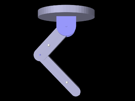
The example model artisynth.demos.tutorial.IKMultiJointedArm shows how to move the MultiJointedArm model (Section 3.5.16) using an IKProbe and marker target data read from a TRC file. This is essentially the same demo as TRCMultiJointedArm (Section 5.5.3), except that it uses inverse kinematics instead of a crude physical simulation in which the markers are connected to the target points by springs. The source code for the build() method is shown below:
Since the model extends MultiJointedArm, build() first calls super.build() to create that model. Next, as in TRCMultiJointedArm, a TRC file containing the marker trajectories is read (lines 5-7). Next, an IKProbe is created to control the markers, with its start and stop times determined directly from the TRC frame times (lines 10-16).
To illustrate a different way of setting probe data, the marker positions for each frame are extracted directly from the TRC reader and added to the probe using addData(t,vec) (lines 19-24). The probe’s bodiesNonDynamicIfActive property is also set (line 27) to ensure that the rigid bodies are set non-dynamic when the probe is active.
To run this example in ArtiSynth, select All demos > tutorial > IKMultiJointedArm from the Models menu.
10.5.5 Example: controlling ToyMuscleArm with inverse kinematics
The final example in this chapter also involves using the tracking controller to move ToyMuscleArm. Several marker targets are used, driven by data read from a TRC file, an IKSolver transforms the data into a feasible trajectory, and the data is used to create velocity targets that when combined with PD control reduce the tracking error. The model is
artisynth.demos.tutorial.IKInverseMuscleArm
and its class definition, excluding import statements, is shown below:
The build() method starts by setting up a tracking controller in the same manner as for InverseMuscleArm (Section 10.2.4) (lines 10-18). Next, the base body is marked as “ground” by setting its grounded property (line 20); this is necessary to prevent the IKSolver from moving it.
This example tracks three markers with component numbers 8, 0, and 2. These are collected into the list markers and added to the controller as targets (lines 20-36). A target position probe containing the marker trajectory, and attached to the tracking controller target points, is then created directly from the TRC file (lines 41-46). Since this file contains data for all the markers, we specify the markers we want using the label list mkrLabels which was created from their numbers.
To filter the marker data (which for this example has been deliberately misregistered), an IKSolver is created and used to create an input probe containing a feasible trajectory (lines 49-51). The data from this probe is then used to overwrite that of the target position probe (line 53). After this is done, the target position probe is differentiated to create a target velocity probe (lines 56-59). To take advantage of this velocity information, the controller is configured to use PD control (lines 62-65) with constants that were tuned manually. Lastly, an output probe is created to record the excitations, and another is created to observe both the target and actual position of the distal marker (which appears first in markers).
To run this example in ArtiSynth, select All demos > tutorial > IKInverseMuscleArm from the Models menu. A view of the timeline, showing the four probes, is given in Figure 10.19. Figure 10.20 (left) shows the resulting excitations, while Figure 10.20 (right) shows the different excitations produced if the target trajectory is left unfiltered. (To run with an unfiltered trajectory, comment out line 53. The model will then appear as in Figure 10.18, right). Finally, Figure 10.21 shows two outputs of the “distal tracking” probe, the left one with velocity information available to the controller, and the right one with it removed (which can be done interactively by making the target velocity probe inactive). Without velocity information, the marker lags the target by a noticeable amount.
10.6 Caveats and limitations
Use of the inverse controller is subject to some caveats.
-
•
Tracked components must be dynamic, in that their motion is controlled by forces. This means that their dynamic property must be set to true or they must be attached to other bodies that are dynamic.
-
•
The algorithm which computes the excitations currently has a complexity
 in the number of excitations . This is due both
to the use of numeric differentiation for determining excitation response
matrices such as and (Section
10.1.3), and also the fact that the QP solver
is at present a dense solver. This means that applications with large numbers
of excitations may require considerably longer to simulate than those with
fewer excitations.
in the number of excitations . This is due both
to the use of numeric differentiation for determining excitation response
matrices such as and (Section
10.1.3), and also the fact that the QP solver
is at present a dense solver. This means that applications with large numbers
of excitations may require considerably longer to simulate than those with
fewer excitations. -
•
The controller is not designed to work with unilateral constraints (the most common examples of which are constraint-based contact and joint limits). For models containing these behaviors, inverse simulation may produce excitations that jump around erratically. In the case of collisions, one solution may be to use force-based collisions, implemented with either PointPlaneForce or PointMeshForce, as described in Section 3.8. Setting these components to use a quadratic force function may improve performance even more. Another possible solution, for any kind of unilateral constraint, may be to make it compliant (Sections 3.4.9 and 8.7), since this has the same effect as making the constraint force-based.
-
•
Prescribed motion trajectories may need to be sufficiently smooth to avoid large transient excitations, particularly at the start and end of motions when velocities transition from and to 0. Transient effects are often more pronounced for models where inertial effects are high. Cubic interpolation is useful for creating smoother trajectories, particularly with a limited number of data points. It may also be necessary to explicitly smooth an input trajectory with additional points.
Chapter 11 Skinning
A useful technique for creating anatomical and biomechanical models is to attach a passive mesh to an underlying set of dynamically active bodies so that it deforms in accordance with the motion of those bodies. ArtiSynth allows meshes to be attached, or “skinned”, to collections of both rigid bodies and FEM models, facilitating the creation of structures that are either embedded in, or connect or envelope a set of underlying components. Such approaches are well known in the computer animation community, where they are widely used to represent the deformable tissue surrounding a “skeleton” of articulated rigid bodies, and have more recently been applied to biomechanics [17].
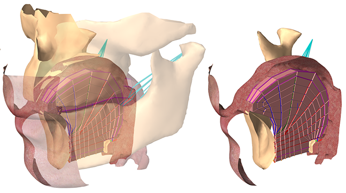
One application of skinning is to create a continuous skin surrounding an underlying set of anatomical components. For example, for modeling the human airway, a disparate set of models describing the tongue, jaw, palate and pharynx can be connected together with a surface skin to form a seamless airtight mesh (Figure 11.1), as described in [25]. This then provides a uniform boundary for handling air or fluid interactions associated with tasks such as speech or swallowing.
ArtiSynth provides support for “skinning” a mesh over an underlying set of master bodies, consisting of rigid bodies and/or FEM models, such that the mesh vertices deform in response to changes in the position, orientation and shape of the master bodies.
11.1 Implementation
This section describes the technical details of the ArtiSynth skinning
mechanism. A skin mesh is implemented using a
SkinMeshBody, which contains a
base mesh and references to a set of underlying dynamic master
bodies. A master body can be either a
Frame (of which
RigidBody is a subclass), or a
FemModel3d. The positions of the
mesh vertices (along with markers and other points that can be
attached to the skin mesh) are determined by a weighted sum of
influences from each of the ![]() master bodies, such that as the latter
move and/or deform, the vertices and attached points deform as
well. More precisely, for each master body
master bodies, such that as the latter
move and/or deform, the vertices and attached points deform as
well. More precisely, for each master body
![]() , let
, let ![]() be the weighting factor and
be the weighting factor and
![]() the connection function that describes the
contribution of body
the connection function that describes the
contribution of body ![]() to the position of the vertices (or attached
points) as a function of its generalized coordinates
to the position of the vertices (or attached
points) as a function of its generalized coordinates ![]() . Then if
the position of a vertex (or attached point) is denoted by
. Then if
the position of a vertex (or attached point) is denoted by ![]() and
its initial (or base) position is
and
its initial (or base) position is ![]() , we have
, we have
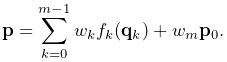 |
(11.1) |
The weight ![]() in the last term is known as the base weight
and describes an optional contribution from the base position
in the last term is known as the base weight
and describes an optional contribution from the base position ![]() .
Usually
.
Usually ![]() , unless the vertex is not connected to any
master bodies, in which case
, unless the vertex is not connected to any
master bodies, in which case ![]() , so that the vertex is anchored
to its initial position.
, so that the vertex is anchored
to its initial position.
In general, connection weights ![]() are computed based on the
distances
are computed based on the
distances ![]() between the vertex (or attached point) and
each master body
between the vertex (or attached point) and
each master body ![]() . More details on this are given in Sections
11.2 and 11.3.
. More details on this are given in Sections
11.2 and 11.3.
For Frame master bodies, the connection function is one associated with various rigid body skinning techniques known in the literature. These include linear, linear dual quaternion, and iterative dual quaternion skinning. Which technique is used is determined by the frameBlending property of the SkinMeshBody, which can be queried or set in code using the methods
where FrameBlending is an enumerated type defined by SkinMeshBody with the following values:
- LINEAR
-
Linear blending, in which the connection function
 implements a
standard rigid connection between the vertex and the frame
coordinates. Let the frame’s generalized coordinates
implements a
standard rigid connection between the vertex and the frame
coordinates. Let the frame’s generalized coordinates  be given
by the
be given
by the  rotation matrix
  and translation vector
  describing its pose, with its initial pose given by
  and
and
 . The connection function then takes the form
(11.2) Linear blending is faster than other blending techniques but is more prone to pinching and creasing artifacts in the presence of large rotations between frames.
- DUAL_QUATERNION_LINEAR
-
Linear dual quaternion blending, which is more computationally expensive but typically gives better results than linear blending, and is described in detail as DLB in [8]. Let the frame’s generalized coordinates
be given by the dual-quaternion
 (describing both rotation and translation), with the
initial pose given by the dual-quaternion
(describing both rotation and translation), with the
initial pose given by the dual-quaternion  . Then define
the relative dual-quaternion
. Then define
the relative dual-quaternion  as
as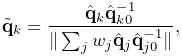
(11.3) where the denominator is formed by summing over all master bodies
 which are frames. The connection function is then
given by
which are frames. The connection function is then
given by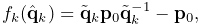
(11.4) where we note that a dual quaternion multiplied by a position vector yields a position vector.
- DUAL_QUATERNION_ITERATIVE
-
Dual quaternion iterative blending, which is a more complex dual quaternion technique described in detail as DIB in [8]. The connection function for iterative dual quaternion blending involves an iterative process and is not described here. It also does not conform to (11.1), because the connection functions
for the Frame master
bodies do not combine linearly. Instead, if there
are Frame master bodies, there is a single
connection function
(11.5) that determines the connection for all of them, given their weighting factors
 and generalized coordinates
  .
Iterative blending relies on two parameters: a blend tolerance, and a
maximum number of blend steps, both of which are controlled by the
SkinMeshBody properties DQBlendTolerance and DQMaxBlendSteps, which have default values of
.
Iterative blending relies on two parameters: a blend tolerance, and a
maximum number of blend steps, both of which are controlled by the
SkinMeshBody properties DQBlendTolerance and DQMaxBlendSteps, which have default values of  and
and  .
.Iterative dual quaternion blending is not completely supported in ArtiSynth. In particular, because of its complexity, the associated force and velocity mappings are computed using the simpler computations employed for linear dual quaternion blending. For the examples shown in this chapter, iterative dual quaternion gives results that are quite close to those of linear dual quaternion blending.
For FEM master bodies, the connection works by tying each vertex (or
attached point) to a specific FEM element using a fixed-length offset
vector ![]() that rotates in conjunction with the element. This is
illustrated in Figure 11.2 for the case of a
single FEM master body. Starting with the initial vertex position
that rotates in conjunction with the element. This is
illustrated in Figure 11.2 for the case of a
single FEM master body. Starting with the initial vertex position
![]() , we find the nearest point
, we find the nearest point ![]() on the nearest FEM
element, along with the offset vector
on the nearest FEM
element, along with the offset vector ![]() . The point
. The point ![]() can be expressed as the weighted
sum of the initial element nodal positions
can be expressed as the weighted
sum of the initial element nodal positions ![]() ,
,
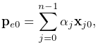 |
(11.6) |
where ![]() is the number of nodes and
is the number of nodes and ![]() represent the
(constant) nodal coordinates. As the element moves and deforms, the
element point
represent the
(constant) nodal coordinates. As the element moves and deforms, the
element point ![]() moves with the nodal positions
moves with the nodal positions ![]() according
to the same relationship, while the offset vector
according
to the same relationship, while the offset vector ![]() rotates
according to
rotates
according to ![]() , where
, where ![]() is the rotation of the
element’s coordinate frame
is the rotation of the
element’s coordinate frame ![]() with respect to its initial
orientation. The connection function
with respect to its initial
orientation. The connection function ![]() then takes the form
then takes the form
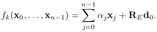 |
(11.7) |
![]() is determined by computing a polar decomposition
is determined by computing a polar decomposition ![]() on the deformation gradient
on the deformation gradient ![]() at the element’s center. We note that
the displacement
at the element’s center. We note that
the displacement ![]() is only rotated and so the distance
is only rotated and so the distance ![]() of the vertex from the element remains constant. If the
vertex is initially on or inside the element, then
of the vertex from the element remains constant. If the
vertex is initially on or inside the element, then ![]() and
(11.7) takes the form of a standard point/element
attachment as described in 6.4.3.
and
(11.7) takes the form of a standard point/element
attachment as described in 6.4.3.
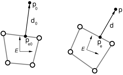
While it is sometimes possible to determine weights
that control a vertex position outside an element, without the need for an offset vector
, the resulting vertex positions tend to be very sensitive to element distortions, particularly when the vertex is located at some distance. Keeping the element-vertex distance constant via an offset vector usually results in more plausible skinning behavior.
11.2 Creating a skin mesh
As mentioned above, skin meshes within ArtiSynth are implemented using the SkinMeshBody component. Applications typically create a skin mesh in code according to the following steps:
-
1.
Create an instance of SkinMeshBody and assign its underlying mesh, usually within the constructor;
-
2.
Add references to the required master bodies;
-
3.
Compute the master body connections
This is illustrated by the following example:
Master body references are added using
addMasterBody().
When all the master bodies have been added, the method
computeAllVertexConnections()
computes the weighted connections to each vertex. The connection
weights ![]() for each vertex are determined by a weighting
function, based on the distances
for each vertex are determined by a weighting
function, based on the distances ![]() between the vertex and each
master body. The default weighting function is inverse-square
weighting, which first computes a set of raw weights
between the vertex and each
master body. The default weighting function is inverse-square
weighting, which first computes a set of raw weights ![]() according to
according to
 |
(11.8) |
where ![]() is the minimum master body distance,
and then normalizes these to determine
is the minimum master body distance,
and then normalizes these to determine ![]() :
:
 |
(11.9) |
Other weighting functions can be specified, as described in Section 11.3.
SkinMeshBody provides the following set of methods to set and query its master body configuration:
When a Frame master body is added using addMasterBody(),
its initial, or base, pose (corresponding to ![]() and
and
![]() in Section 11.1) is set from its
current pose. If necessary, applications can later query and reset
the base pose using the methods getBasePose() and setBasePose().
in Section 11.1) is set from its
current pose. If necessary, applications can later query and reset
the base pose using the methods getBasePose() and setBasePose().
Internally, each vertex is connected to the master bodies by a
PointSkinAttachment, which
contains a list
of
PointSkinAttachment.SkinConnection
components describing each master connection. Applications can obtain
the PointSkinAttachment for each vertex using the method
where vidx is the vertex index, which must be in the range 0 to
numv-1, with numv the number of vertices as returned by
numVertices(). Methods also exist to query and set each
vertex’s base (i.e., initial) position ![]() :
:
11.2.1 Example: skinning over rigid bodies
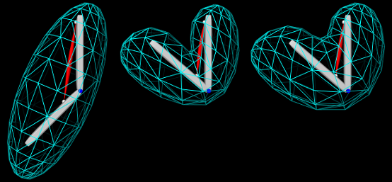
.
An example of skinning a mesh over two rigid bodies is given by artisynth.demos.tutorial.RigidBodySkinning. It consists of a SkinMeshBody placed around two rigid bodies connected by a hinge joint to form a toy “arm”, with a Muscle added to move the lower body with respect to the upper. The code for the build() method is given below:
A MechModel is created in the usual way (lines 2-7). To this is added a very simple toy “arm” consisting of an upper and lower body connected by a hinge joint (lines 9-27), with a simple point-to-point muscle attached between frame markers on the upper and lower bodies to provide a means of moving the arm (lines 29-36). Creation of the arm bodies uses an addBody() method which is not shown.
The mesh to be skinned is an ellipsoid, created using the FemFactory method createSphere() to produce a spherical mesh which is then scaled and repositioned (lines 38-43). The skin body itself is then created around this mesh, with the upper and lower bodies assigned as master bodies and the connections computed using computeAllVertexConnections() (lines 45-50).
A control panel is added to allow control over the muscle’s excitation as well as the skin body’s frameBlending property (lines 52-56). Finally, render properties are set (lines 58-67): the skin mesh is made transparent by setting its faceStyle and drawEdges properties to NONE and true, respectively, with cyan colored edges; the muscle is rendered as a red spindle; the joint is drawn as a blue cylinder and the bodies are colored light gray.
To run this example in ArtiSynth, select All demos > tutorial > RigidBodySkinning from the Models menu. The model should load and initially appear as in Figure 11.3 (left). When running the simulation, the arm can be flexed by adjusting the muscle excitation property in the control panel, causing the skin mesh to deform (Figure 11.3, middle). Changing the frameBlending property from its default value of LINEAR to DUAL_QUATERNION_LINEAR causes the mesh deformation to become fatter and less prone to creasing (Figure 11.3, right).
11.3 Computing weights
As described above, the default method for computing skin connection weights is inverse-square weighting (equations 11.8 and 11.9). However, applications can specify alternatives to this. The method
causes weights to be computed according to a Gaussian weighting
scheme, with sigma specifying the standard deviation ![]() .
Raw weights
.
Raw weights ![]() are then computed according to
are then computed according to
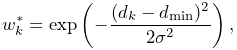 |
and then normalized to form ![]() .
.
The method
reverts the weighting function back to inverse-square weighting.
It is also possible to specify a custom weighting function by implementing a subclass of SkinWeightingFunction. Subclasses must implement the function
in which the weights for each master body are computed and returned in weights. pos gives the initial position of the vertex (or attached point) being skinned, while nearestPnts provides information about the distance from pos to each of the master bodies, using an array of SkinMeshBody.NearestPoint objects:
Once an instance of SkinWeightingFunction has been created, it can be set as the skin mesh weighting function by calling
Subsequent calls to computeAllVertexConnections(), or the addMarker or computeAttachment methods described in Section 11.4, will then employ the specified weighting.
As an example, imagine an application wishes to compute weights according to an inverse-cubic weighting function, such that
 |
A subclass of SkinWeightingFunction implementing this could then be defined as
and then set as the weighting function using the code fragment:
The current weighting function for a skin mesh can be queried using
The inverse-square and Gaussian weighting methods described above are implemented using the system-provided SkinWeightingFunction subclasses InverseSquareWeighting and GaussianWeighting, respectively.
11.3.1 Setting weights explicitly
As an alternative to the weighting function, applications can also create connections to vertices or points in which the weights are explicitly specified. This allows for situations in which a weighting function is unable to properly specify all the weights correctly.
When a mesh is initially added to a skin body, via either the constructor SkinMeshBody(mesh), or by a call to setMesh(mesh), all master body connections are cleared and the vertex position is “fixed” to its initial position, also known as its base position. After the master bodies have been added, vertex connections can be created by calling computeAllVertexConnections(), as described above. However, connections can also be created on a per-vertex basis, using the method
where vidx is the index of the desired vertex and weights is an optional argument which if non-null explicitly specifies the connection weights. A sketch example of how this can be used is given in the following code fragment:
For comparison, it should be noted that the code fragment
in which weights are not explicitly specified, is equivalent to calling computeAllVertexConnections().
If necessary, after vertex connections have been computed, they can also be cleared, using the method
This will disconnect the vertex with index vidx from the master
bodies, and set its base weighting ![]() (equation
11.1) to 1, so that it will remain fixed to its initial
position.
(equation
11.1) to 1, so that it will remain fixed to its initial
position.
In some special cases, it may be desirable for an application to set attachment base weights to some value other than 0 when connections are present. Base weights for vertex attachments can be queried and set using the methods
In the second method, the argument normalize, if true, causes the weights of the other connections to be scaled so that the total weight sum remains the same. For skin markers and point attachments (Section 11.4), base weights can be set by calling the equivalent PointSkinAttachment methods
(If needed, the attachment for a skin marker can be obtained by
calling its getAttachment() method.) In addition, base weights
can also be specified in the weights argument to the method computeVertexConnections(vidx,weights), as well as the methods addMarker(name,pos,weights) and createPointAttachment(pnt,weights) described in Section
11.4. This is done by giving weights
a size equal to ![]() , where
, where ![]() is the number of master bodies, and
specifying the base weight in the last location.
is the number of master bodies, and
specifying the base weight in the last location.
11.4 Markers and point attachments
In addition to controlling the positions of mesh vertices, a SkinMeshBody can also be used to control the positions of dynamic point components, including markers and other points which can be attached to the skin body. For both markers and attached points, any applied forces are propagated back onto the skin body’s master bodies, using the principle of virtual work. This allows skin bodies to be fully incorporated into a dynamic model.
Markers and point attachments can be created even if the SkinMeshBody does not have a mesh, a fact that can be used in situations where a mesh is unnecessary, such as when employing skinning techniques for muscle wrapping (Section 11.7).
11.4.1 Markers
Markers attached to a skin body are instances of SkinMarker, and are contained in the body’s subcomponent list markers (analogous to the markers list for FEM models). Markers can be created and maintained using the following SkinMeshBody methods:
The addMarker methods each create and return a SkinMarker which is added to the skin body’s list of markers. The marker’s initial position is specified by pos, while the second and third methods also allow a name to be specified. Connections between the marker and the master bodies are created in the same way as for mesh vertices, with the connection weights either being determined by the skin body’s weighting function (as returned by getWeightingFunction()), or explicitly specified by the argument weights (third method).
Once created, markers can be removed individually or all together by the removeMarker() and clearMarkers() methods. The entire marker list can be accessed on a read-only basis by the method markers().
11.4.2 Point attachments
In addition to markers, applications can also attach any regular Point component (including particles and FEM nodes) to a skin body by using one of its createPointAttachment methods:
Both of these create a PointSkinAttachment that connects the point pnt to the master bodies in the same way as for mesh vertices and markers, with the connection weights either being determined by the skin body’s weighting function or explicitly specified by the argument weights in the second method.
Once created, the point attachment must also be added to the underlying MechModel, as illustrated by the following code fragment:
11.4.3 Example: skinning rigid bodies and FEM models
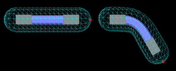
An example of skinning a mesh over both rigid bodies and FEM models is
given by the demo model
artisynth.demos.tutorial.AllBodySkinning. It consists
of a skin mesh placed around a tubular FEM model
connected to rigid bodies connected at each end, and a
marker attached to the mesh tip.
The code for the build() method is given below:
A MechModel is first created and length and density parameters
are defined (lines 2-8). Then a tubular FEM model is created, by using
the FemFactory method createHexTube() and transforming the result by rotating it by 90
degrees about the ![]() axis (lines 10-14). Two rigid body blocks are
then created (lines 16-26) and attached to the ends of the FEM model
by finding and attaching the left and rightmost nodes (lines 28-34).
The model is anchored to ground by setting the left block to be
non-dynamic (line 21).
axis (lines 10-14). Two rigid body blocks are
then created (lines 16-26) and attached to the ends of the FEM model
by finding and attaching the left and rightmost nodes (lines 28-34).
The model is anchored to ground by setting the left block to be
non-dynamic (line 21).
The mesh to be skinned is a rounded cylinder, created using the
MeshFactory method createRoundedCylinder() and rotating the result by 90 degrees about
the ![]() axis (lines 39-44). This is then used to create the skin body
itself, to which both rigid bodies and the FEM model are added as
master bodies and the vertex connections are computed using a call to
computeAllVertexConnections() (lines 46-52). A marker is then
added to the tip of the skin body, using the addMarker() method
(lines 54-56). Finally render properties are set (lines 58-64):
The mesh is made transparent by drawing only its edges in cyan; the
FEM model surface mesh is rendered in blue-gray, and the
tip marker is drawn as a red sphere.
axis (lines 39-44). This is then used to create the skin body
itself, to which both rigid bodies and the FEM model are added as
master bodies and the vertex connections are computed using a call to
computeAllVertexConnections() (lines 46-52). A marker is then
added to the tip of the skin body, using the addMarker() method
(lines 54-56). Finally render properties are set (lines 58-64):
The mesh is made transparent by drawing only its edges in cyan; the
FEM model surface mesh is rendered in blue-gray, and the
tip marker is drawn as a red sphere.
To run this example in ArtiSynth, select All demos > tutorial > AllBodySkinning from the Models menu. The model should load and initially appear as in Figure 11.4 (left). When running the simulation, the FEM and the rightmost rigid body fall under gravity, causing the skin mesh to deform. The pull tool can then be used to move things around by applying forces to the master bodies or the skin mesh itself.
11.4.4 Mesh-based markers and attachments
For the markers and point attachments described above, the connections to the underlying master bodies are created in the same manner as connections for individual mesh vertices. This means that the resulting markers and attached points move independently of the mesh vertices, as though they were vertices in their own right.
An advantage to this is that such markers and attachments can be created even if the SkinMeshBody does not even have a mesh, as noted above. However, a disadvantage is that such markers will not remain tightly connected to vertex-based features (such as the faces of a PolygonalMesh or the line segments of a PolylineMesh). For example, consider a marker defined by
where pos is a point that is initially located on a face of the body’s mesh. As the master bodies move and the mesh deforms, the resulting marker may not remain strictly on the face. In many cases, this may not be problematic or the deviation may be too small to matter. However, if it is desirable for markers or point attachments to be tightly bound to mesh features, they can instead be created with the following methods:
The requested position pos will then be projected onto the
nearest mesh feature (e.g., a face for a PolygonalMesh or a line
segment for a PolylineMesh), and the resulting position ![]() will be defined as a linear combination of the vertex positions
will be defined as a linear combination of the vertex positions
![]() for this feature,
for this feature,
| (11.10) |
where ![]() are the barycentric coordinates of
are the barycentric coordinates of ![]() with respect
to the feature. The master body connections are then defined by the
same linear combination of the connections for each vertex. When the
master bodies move, the marker or attached point will move with the
feature and remain in the same relative position.
with respect
to the feature. The master body connections are then defined by the
same linear combination of the connections for each vertex. When the
master bodies move, the marker or attached point will move with the
feature and remain in the same relative position.
Since SkinMeshBody implements the interface PointAttachable, it provides the general point attachment method
which allows it to be acted on by agents such as the ArtiSynth marker tool (see the section “Marker tool” in the ArtiSynth User Interface Guide). Whether or not the resulting attachment is a regular attachment or mesh-based is controlled by the skin body’s attachPointsToMesh property, which can be adjusted in the GUI or in code using the property’s accessor methods:
11.5 Resolution and Limitations
Skinning techniques do have limitations, which are common to all methodologies.
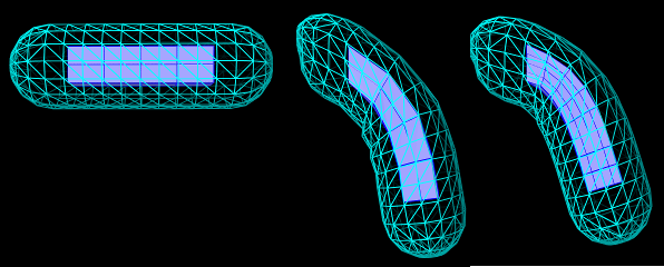
-
•
The passive nature of the connection between skinned vertices and the master bodies means that it can be easy for the skin mesh to self intersect and/or fold and crease in ways that are not physically realistic. These effects are often more pronounced when mesh vertices are relatively far away from the master bodies, or in places where the mesh undergoes a concave deformation. When the master bodies include frames, these effects can sometimes be reduced by setting the frameBlending property to DUAL_QUATERNION_LINEAR instead of the default LINEAR.
-
•
When the master bodies include FEM models which undergo large deformations, crimping artifacts may arise if the skin mesh has a higher resolution than the FEM model (Figure 11.5). This is because each mesh vertex is connected to the coordinate frame of a single FEM element, and for reasons of computational efficiency the influence of these coordinate frames is not blended as it is for frame-based master bodies. If crimping artifacts occur, one solution may be to adjust the mesh and/or the FEM model so that their resolutions are more compatible (Figure 11.5, right).
11.6 Collisions
It is possible to make skin bodies collide with other ArtiSynth bodies, such as RigidBody and FemModel3d, which implement the Collidable interface (Chapter 8). SkinMeshBody itself implements CollidableBody, and is considered a deformable body, so that collisions can be activated either by setting one of the default collision behaviors involving deformable bodies, or by setting an explicit collision behavior between it and another body. Self collisions involving SkinMeshBody are not currently supported.
As described in Section 8.4, collisions work by computing the intersection between the meshes of the skin body and other collidables. The vertices, faces, and (possibly) edges of the resulting intersection region are then used to compute contact constraints, which propagate the effect of the contact back onto the collidable bodies’ dynamic components. For a skin mesh, the dynamic components are the Frame master bodies and the nodes of the FEM master bodies.
Collisions involving SkinMeshBody frequently suffer from the problem of being overconstrained (Section 8.6), whereby the number of contacts exceeds the number of master body DOFs available to handle the collision. This may occur if the skin body contains only rigid bodies, or if the mesh resolution exceeds the resolution of the FEM master bodies. Managing overconstrained collisions is discussed in Section 8.6, with the easiest method being constraint reduction, which can be activated by setting to true the reduceConstraints property for either the collision manager or a specific CollisionBehavior involving the skin body.
Caveats: The distance between the vertices of a skinned mesh and its master bodies can sometimes cause odd or counter-intuitive collision behavior. Collision handling may also be noticeably slower if frameBlending is set to DUAL_QUATERNION_LINEAR or DUAL_QUATERNION_ITERATIVE. If any of the master bodies are FEM models, collisions resulting in large friction forces may result in unstable behavior.
11.6.1 Example: collision with a cylinder
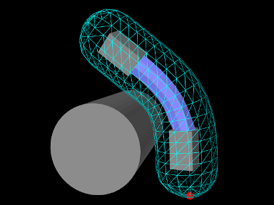
Collisions involving SkinMeshBody are illustrated by the demo model artisynth.demos.tutorial.SkinBodyCollide, which extends the demo AllBodySkinning to add a cylinder with which the skin body can collide. The code for the demo is given below:
The model subclasses AllBodySkinning, using the superclass build() method within its own build() method to create the original model (line 12). It then obtains references to the MechModel, SkinMeshBody, and leftmost block, using their names to find them in various component lists (lines 14-17). (If the original model had stored references to these components as accessible member attributes, this step would not be needed.)
These component references are then used to make changes to the model: the left block is made dynamic so that the skin mesh can fall freely (line 21), a cylinder is created and added (lines 23-30), collisions are enabled between the skin body and the cylinder (lines 32-34), and the collision manager is asked to use constraint reduction to minimize the chance of overconstrained contact (line 35).
To run this example in ArtiSynth, select All demos > tutorial > SkinBodyCollide from the Models menu. When run, the skin body should fall and collide with the cylinder as shown in Figure 11.6.
11.7 Application to muscle wrapping
It is sometimes possible to use skinning as a computationally cheaper way to implement muscle wrapping (Chapter 9).
Typically, the end points (i.e., origin and insertion points) of a point-to-point muscle are attached to different bodies. As these bodies move with respect to each other, the path of the muscle may wrap around portions of these bodies and perhaps other intermediate bodies as well. The wrapping mechanism of Chapter 9 manages this by performing the computations necessary to allow one or more wrappable segments of a MultiPointSpring to wrap around a prescribed set of rigid bodies. However, if the induced path deformation is not too great, it may be possible to achieve a similar effect at much lower computational cost by simply “skinning” the via points of the multipoint spring to the underlying rigid bodies.
The general approach involves:
-
1.
Creating a SkinMeshBody which references as master bodies the bodies containing the origin and insertion points, and possibly other bodies as well;
-
2.
Creating the wrapped muscle using a MultiPointSpring with via points that are attached to the skin body.
It should be noted that for this application, the skin body does not need to contain a mesh. Instead, “skinning” connections can be made solely between the master bodies and the via points. An easy way to do this is to simply use skin body markers as via points. Another way is to create the via points as separate particles, and then attach them to the skin body using one of its createPointAttachment methods.
It should also be noted that unlike with the wrapping methods of Chapter 9, skin-based wrapping can be applied around FEM models as well as rigid bodies.
Generally, we observe better wrapping behavior if the frameBlending property of the SkinMeshBody is set to DUAL_QUATERNION_LINEAR instead of the default value of LINEAR.
11.7.1 Example: wrapping for a finger joint
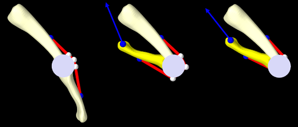
An example of skinning-based muscle wrapping is given by artisynth.demos.tutorial.PhalanxSkinWrapping, which is identical to the demo artisynth.demos.tutorial.PhalanxWrapping except for using skinning to achieve the wrapping effect. The portion of the code which differs is shown below:
First, a SkinMeshBody is created referencing the proximal and distal bones as master bodies, with the frameBlending property set to DUAL_QUATERNION_LINEAR (lines 1-6). Next, we create a set of three via points that will be attached to the skin body to guide the muscle around the joint in lieu of making it actually wrap around a cylinder (lines 7-9).
In the original PhalanxWrapping demo, a RigidCylinder was used as a muscle wrap surface. In this demo, we replace this with a simple cylindrical mesh which has no dynamic function but allows us to visualize the wrapping behavior of the via points (lines 11-18). The muscle itself is created using the three via points but with no wrappable segments or bodies (lines 20-30).
A control panel is added to allow for the adjustment of the skin body’s frameBlending property (lines 32-35). Finally, render properties are set as for the original demo, only with the skin body markers rendered as white spheres to make them more visible (lines 37-41).
To run this example in ArtiSynth, select All demos > tutorial > PhalanxSkinWrapping from the Models menu. The model should load and initially appear as in Figure 11.7 (left). The pull tool can then be used to move the distal joint while simulating, to illustrate how well the via points “wrap” around the joint, using the cylindrical mesh as a visual reference (Figure 11.7, middle). Changing the frameBlending property to LINEAR results in a less satisfactory behavior (Figure 11.7, right).
Chapter 12 Importing OpenSim Models
12.1 Overview
ArtiSynth provides an OpenSimParser class that can be used to import parts of an OpenSim model ([7]; versions 3 or 4), translating the components into their ArtiSynth equivalents and arranging them inside a MechModel. The OpenSim component hierarchy is preserved, and the resulting MechModel components can be queried using methods supplied by the parser. Not all OpenSim components are implemented, but those that are include most of the commonly used components found in "bodyset", "jointset", "forceset", "constraintset", and "markerset". Implemented muscles include Thelen2003Muscle and Millard2012EquilibriumMuscle.
By using this parser, applications may leverage the large existing corpus of OpenSim models as a starting point for ArtiSynth models. As usual, model creation is done inside the model’s build() method, and typically entails the following steps:
-
1.
Use OpenSimParser to import the OpenSim model into a corresponding MechModel.
-
2.
Understand the component hierarchy that realizes the model.
-
3.
Adjust the visualization and tune parameters if needed so the model is stable under forward simulation.
-
4.
Edit the model by removing unneeded components and/or adding structures, such as FEM models, not present in the original.
These steps will now be discussed in more detail.
12.2 Importing the OpenSim model
To import an OpenSim model, an application uses the class OpenSimParser. Its primary constructor is
| OpenSimParser (File osimFile, File geometryPath) |
where osimFile references the .osim file and geometryPath references the folder where the geometry is located. If geometryPath is specified as null, the parser will look for the geometry under either "Geometry" or "geometry", in the same folder as the .osim file.
After creating the parser, the model can be loaded by calling createModel(), which reads the model file, generates the equivalent ArtiSynth components, and arranges them in the specified MechModel:
If the mech argument is null, createModel() generates a fresh MechModel and returns it.
The listing below shows a complete example given in
artisynth.demos.opensim.OpenSimArm26
which imports the Arm26 model by Reinbolt, Seth, Habib, and Hamner, and based on an earlier model by Kate Holzbaur.
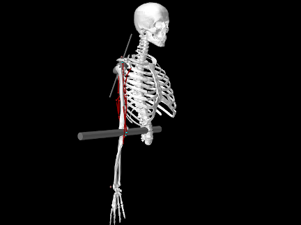
When loaded into ArtiSynth, the model appears as in Figure 12.1. The OpenSim model contains a number of components that are not implemented by ArtiSynth, as seen by the console messages
OpenSimParser: ignoring ControllerSet OpenSimParser: ignoring ContactGeometrySet OpenSimParser: ignoring ProbeSet
After calling createModel(), the build() method changes the view orientation, sets damping for the rigid bodies, and creates control panels to adjust the excitations and joint coordinates. These are actions described further in Section 12.4.
12.3 The component hierarchy
OpenSimParser arranges implementing components within MechModel in a manner that preserves the hierarchy and naming of the original OpenSim model. This results in a component hierarchy different from the canonical one used by MechModel, in which components are placed in container lists by type (e.g., particles in a PointList<Particle> named "particles", rigid bodies in a RenderableComponentList<RigidBody> named "rigidBodies", axial springs in an AxialSpringList<AxialSpring> list named "axialSprings"). However, as described in Section 4.8, applications are free to create custom component arrangements, and OpenSimParser does this, recreating the basic OpenSim containers "bodyset", "jointset" (for OpenSim 4), "forceset", "constraintset" and "markerset". Figure 12.2 illustrates this by showing the ArtiSynth navigation panel for the OpenSimArm26 example. The only original MechModel component that appears is the collisionManager (the other canonical containers, such as "particles", "rigidBodies", etc., are still present, but don’t appear because they are empty).
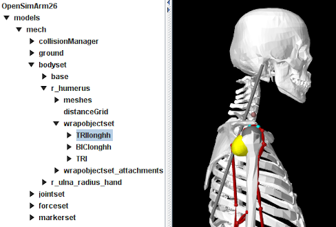
12.3.1 Ground
If present, the OpenSim 4 "ground" component appears as its own component, implemented using a RigidBody whose dynamic property is set false and grounded property is set true.
12.3.2 Body set
The body set is implemented as a RenderableComponentList<RigidBody>, with each body implemented by a special implementation of RigidBody that contains a child component named "wrapobjectset" that in turn contains any attached wrap objects. Wrap objects themselves are implemented by special instances of RigidBody that implement the WrapComponent interface. Figure 12.2 shows the navigation panel with the body r_humerus expanded and the wrap object TRIlonghh selected. Other body components include meshes and distancegrid, which are defined for all ArtiSynth rigid bodies, and wrapobjectset_attachments, which are the internal attachments connecting the wrap objects to the body.
For OpenSim 3 models, each body also contains a child component "joint", containing the single joint for which that body is the parent. This is in place of the joint set provided by OpenSim 4.
12.3.3 Joint set
For OpenSim 4, the joint set is implemented as a RenderableComponentList<JointBase> containing JointBase components realizing the various OpenSim joints. Custom joints, in particular, are implemented by OpenSimCustomJoint.
12.3.4 Force set
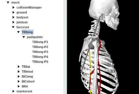
The force set is implemented as a RenderableComponentList<ModelComponent> containing all the supported force effectors. Bushings and CoordinateLimitForces are realized using FrameSpring and JointLimitForce. CoordinateActuators are implemented using JointActuator, while PointToPointActuator is implemented using a custom component TwoPointActuator. Muscles and point-to-point springs are implemented using a special implementation of MultiPointMuscle that contains a child component named "pathpoints" that in turn contains all the muscle’s path points. Each path point is usually a FrameMarker attached to one of the bodies in the body set. Figure 12.3 shows the navigation panel with the muscle TRIlong selected and also expanded to show the path points.
Currently supported OpenSim muscles include Thelen2003Muscle and Millard2012EquilibriumMuscle, which are implemented using the MultiPointMuscle materials Thelen2003AxialMuscle and Millard2012AxialMuscle (Section 4.5.4). All other OpenSim muscles are implemented as a generic instance of ConstantAxialMuscle (Section 4.5.1) whose maxForce property is set to the specified max_isometric_force.
12.3.5 Constraint set
The constraint set is implemented as a ComponentList<ConstrainerBase> containing all the supported constrainers. At present, these include CoordinateCouplerConstraint and PointConstraint, realized by JointCoordinateCoupling and SphericalJoint, respectively.
12.3.6 Marker set
The marker set is implemented as a PointList<Marker> with each marker realized using FrameMarker.
12.4 Inspecting and tuning the model
12.4.1 Visualization
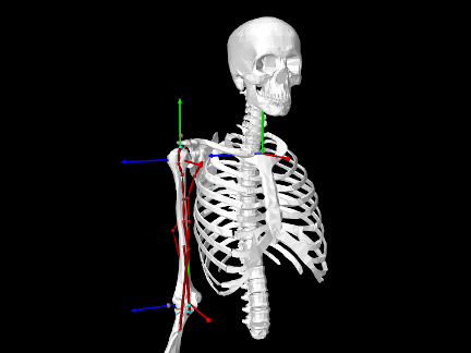
ArtiSynth makes an attempt to preserve the visualization characteristics of the original OpenSim model, but this is not guaranteed. The rendering and appearance of all components can be customized, either interactively (as described under “Editing Properties” in the ArtiSynth User Interface Guide), or in code, as discussed in Section 4.3.
The “frame geometry” associated with OpenSim bodies is not explicitly supported, because ArtiSynth rigid bodies and frames already have a visualization mechanism for their coordinate axes through their axisLength and axisDrawStyle properties. The same is true for wrap objects, which are realized as rigid bodies connected to their parent body via a frame attachment.
OpenSimParser does provide the following convenience methods to control the visibility and coordinate frame rendering of bodies and wrap objects:
| void setBodyFramesVisible (AxisDrawStyle style, double axisLen) |
Set axis rendering for bodies. |
| void setWrapObjectFramesVisible (AxisDrawStyle style, double axisLen) |
Set axis rendering for wrap objects. |
| void setWrapObjectsVisible (boolean visible) |
Set visibility of all wrap objects. |
The last method is supplied to control the collective visibility of all wrap objects since they are distributed among the bodies and can be tedious to access individually. (The collective visibility of bodies, joints, forces, etc. can be controlled by setting the visibility of the containers "bodyset", "jointset", "forceset", etc.)
Placing the following code at the end of the OpenSimArm26 example causes the model to appear as in Figure 12.4:
Wrap object visibility for individual muscles can also be controlled using MultiPointSpring methods:
| boolean hasVisibleWrappables() |
Has wrappables that are currently visible. |
| boolean hasInvisibleWrappables() |
Has wrappables that are currently not visible. |
| void setWrappablesVisible (boolean visible) |
Set the spring’s wrappables to be visible or invisible. |
For information on how to find individual muscles within the model, see Section 12.5.1.
For observing the behavior of joints, it is often useful to display the axes of their C and D coordinate frames. As described in Section (3.4.11), this can be controlled by the joint properties drawFrameC, drawFrameD, and axisLength, which can be set either in code or interactively (by selecting the joint and choosing Edit properties ... from the context menu).
Finally, the coordinate system for OpenSim models is usually arranged with the
![]() axis vertical, whereas ArtiSynth defaults to the
axis vertical, whereas ArtiSynth defaults to the ![]() axis vertical. While
OpenSimParser will set gravity to whatever is specified in the OpenSim
file, the viewer orientation must be set by the application, using the root
model method setDefaultViewOrientation():
axis vertical. While
OpenSimParser will set gravity to whatever is specified in the OpenSim
file, the viewer orientation must be set by the application, using the root
model method setDefaultViewOrientation():
12.4.2 Interactive control panels
As discussed in Section 5.1, applications can create control panels to interactively adjust the values of various component properties. (Properties panels for one or more components can also be created on demand by selecting the components then choosing Edit properties ... from the context menu.)
Also, as shown in the example OpenSimArm26, OpenSimParser provides convenience methods to create two types of control panel:
-
•
CoordinatePanels (Section 5.1.4) to adjust joint coordinate values.
-
•
Control panels to adjust muscle excitations.
The methods are:
| CoordinatePanel createCoordinatePanel() |
Create panel for all coordinates. |
| CoordinatePanel createCoordinatePanel (Collection<JointBase> joints) |
Create panel for specified joints. |
| CoordinatePanel createCoordinatePanel (String[] coordNames) |
Create panel for named coordinates. |
| ControlPanel createExcitationPanel () |
Create panel for all muscles. |
| ControlPanel createExcitationPanel (String[] muscleNames) |
Create panel for named muscles. |
At present, CoordinatePanels do not support the adjustment of other coordinate properties, such as locking or ranges. However, these can set in code (Section 3.4.5), and some can also be set interactively by selecting the joint and opening its property panel.
12.4.3 Model tuning
We recommend testing the model by running it under forward simulation to ensure that it behaves as expected. Some parameters, particularly those relative to damping, may need to be adjusted. There are several steps to this process.
-
•
Check joint function and damping. Remove all force effectors and let the model fall under gravity. If the body is not connected to ground, select an appropriate body and set its dynamic property to false. Force effectors can be removed by selecting the "forceset" and choosing Delete in the context menu; this can also be done in code, as described in Section 12.5.2.
With all force effectors removed, any model instability almost certainly reflects a problem involving either bodies with zero inertia, or bodies that are overconstrained. Both situations will result in a “perturbed pivots” message like the following appearing on the console output:
Pardiso: num perturbed pivots=3
If this occurs, try to isolate the problem by selectively removing joints and/or bodies. This can be done interactively by selecting them in the viewer or navigation panel and choosing Delete from the context menu. Components can also be removed in code, as per Section 12.5.2. Issues sometimes arise over the “ground” body, which OpenSim uses to represent ground (ArtiSynth does not require a ground body). In OpenSim 3 models, where ground is not an explicit component, one should ensure that its dynamic property is set to false.
Stability issues may arise for bodies which are very small or can rotate quite quickly. This can sometimes be addressed by specifying more damping (and sometimes rotaryDamping specifically) for these bodies. Alternatively, one may wish to reduce the simulation step size, from the default of 0.01 sec down to values around 0.001 or possibly lower. This can be interactively adjusted in the GUI, and once a suitable value is found, set in code using the root model’s setMaxStepSize():
setMaxStepSize (0.001);In addition to gravity, you can also use the pull controller (see “Pull manipulation” in the ArtiSynth User Interface Guide) to apply point forces to the various bodies. The main point of the exercise is to see how the model behaves under gravity-like loads, and adjust the damping parameters (Section 3.1.6) so that bodies come to rest after an appropriate time. Critical, or slightly sub-critical, damping can usually be achieved by setting the inertial damping for the MechModel to values in the range of 1-5, but sometimes one may want to adjust damping for specific bodies, or also specify rotary or frame damping.
Damping in an ArtiSynth model is typically applied directly to its particles and rigid bodies, and reflects the fact that body poses and velocities, instead of joint coordinates and speeds, are the primary means of specifying the model’s dynamic state. OpenSim models often specify damping using CoordinateLimitForces; one may wish to remove or limit the use of those components in ArtiSynth. Likewise, one may wish to reduce the use of damping in the muscle forces.
-
•
Check the muscle wrapping. Using a coordinate panel (Section 12.4.2), adjust the coordinates and check that the muscle wrapping appears correct. Issues that can sometimes arise include the path failing to pass through small torus wrap objects, or not wrapping smoothly around cylinders with radii due to insufficient knots in the wrap path.
If a muscle contains wrap objects, they can be made visible or invisible within the GUI by selecting the muscle and then choosing Show wrappables or Hide wrappables from the context menu.
Wrap path issues can usually be fixed by resetting the initialization points and/or number of knots for the problematic wrap segments, using the methods set/getNumKnots() and set/getInitializingPoints() described in Section 9.2. For example, the following code might fix wrapping for a certain segment:
MultiPointSpring spr = (MultiPointSpring)myParser.findMuscle ("BIClong");int segIdx = 1; // index of problematic segmentPoint3d xpnt; // extra point to help initialize the wrap path...spr.setNumKnots (segIdx, 30); // increase number of knots to 30spr.setInitializingPoints ( // reset initializing pointssegIdx, new Point3d[] { xpnt } );spr.updateWrapSegments();The code makes use of the parser method findMuscle(), described in Section 12.5.1.
-
•
Check quiescent and excited model behavior. Start by checking the behavior of the model with no loads or muscle excitations. The purpose of this exercise is to make sure that the model is stable in a “rest” state. Instability here will usually be the result of force effectors that are generating forces that are too large for some reason. As when inspecting the joint-body behavior, one should attempt to isolate the problem by selectively removing components.
OpenSim muscles are sometimes configured with small non-zero initial excitations, in order to facilitate the solution of muscle-tendon equilibrium. ArtiSynth does not require this for its equilibrium muscle implementation, and so applications are free to set muscle excitations to zero. OpenSimParser supplies the convenience method zeroMuscleExcitations() for doing this.
When forces are highly non-linear, stable model behavior may require reducing the step size, as already described for body-joint calibration. It may also be necessary to change the MechModel’s stabilization property from GlobalMass to GlobalStiffness:
import artisynth.core.mechmodels.MechSystemSolver.PosStabilization;...myMech.setStabilization (PosStabilization.GlobalStiffness);(GlobalStiffness is not the default setting because it increases computation time).
A problem we have seen several times involves improper parameter settings for OpenSim’s CoordinateLimitForce component, which is used to implement both soft coordinate limits and coordinate damping. Rotational units for this component are given in degrees (vs. radians for most other OpenSim components). Modelers have sometimes not noticed this, leading to range limits that are either far too small, or stiffness and damping values that are far too high.
After checking the quiescent behavior, use a muscle excitation panel to check that the model reacts as expected (and remains stable) when different muscles are excited. In some cases, it may be desirable to adjust the muscle parameters. For example, the rest lengths for a muscle implemented using Millard2012AxialMuscle could be adjusted as follows:
import artisynth.core.materials.Millard2012AxialMuscle;...double optl, tslack; // new opt fibre length and tendon slack length values...// find problematic muscleMultiPointSpring spr = (MultiPointSpring)myParser.findMuscle ("BIClong");Millard2012AxialMuscle mmat = (Millard2012AxialMuscle)spr.getMaterial();// adjust the materialmmat.setOptFibreLength (optl);mmat.setTendonSlackLength (tslack);Another useful debugging technique can be to temporarily replace the muscle material for problematic muscles with an instance of SimpleAxialMuscle (Section 4.5.1.1):
// replace material for problematic muscleMultiPointSpring spr = (MultiPointSpring)myParser.findMuscle ("BIClong");spr.setMaterial (new SimpleAxialMuscle (/*stiffness*/0, /*damping*/0, /*maxForce*/100));If set with a given maxForce and 0 stiffness and damping, a SimpleAxialMuscle material configures a muscle so that its tension is simply equal to its excitation times maxForce.
12.5 Model editing
Once an OpenSim model has been imported into ArtiSynth and tuned, users will typically want to modify it. This entails locating various OpenSim components, which are then removed, modified or connected to other ArtiSynth components, such as FEM models.
12.5.1 Finding components
Locating the OpenSim components can done in several ways. First, as with all ArtiSynth models, any component that is a descendant of a container component can be found by specifying its path name with respect to the container, using findComponent() method. For example, the MultiPointMuscle TRIlong seen in Figure 12.3 could be obtained using
where we know a priori that the sought component is a MultiPointMuscle and so are comfortable casting it to such. Likewise, the immediate children of any composite component can be accessed using get(idx) or get(name).
Second, most ArtiSynth container classes implement the java.util interfaces Collection<C> and Iterable<C> with respect to their component type C, making list iteration easy:
Finally, OpenSimParser provides a number of methods for finding components after the model has been created:
The following should be noted about these methods:
-
•
For OpenSim 3 models, getGround() and getJointSet() will both return null. To obtain a list of all joints in this case, one can use getJoints(), which collects all joints regardless of where they are located within the hierarchy.
-
•
Access to joint coordinates is provided by means of a JointCoordinateHandle, which encapsulates the information about both the coordinate and the joint to which it belongs.
-
•
The muscles and axial spring components returned by getMusclesAndSprings() are a subset of the components returned by getForceComponents().
12.5.2 Removing components
For component removal, most container classes supply remove() methods that allow this to be done directly. However, care must be taken that other model components either do not have a hard dependency on those being removed, or that the dependent components are removed as well. For example, any muscle component has a hard dependency on the frame markers that serve as its origin and insertion points, so removing either of these markers necessitates removing the muscle as well. The easiest way to ensure the removal of one or more components and their dependencies is to use the utility methods
| void ComponentUtils.deleteComponentAndDependencies (ModelComponent comp) | |
| void ComponentUtils.deleteComponentsAndDependencies (Collection<? extends ModelComponent> comps) | |
For example, to remove a frame marker, one may call
In addition to removing components with hard dependencies, these methods also take care of soft dependencies, by which some components adjust themselves if certain components are deleted. For example, a MultiPointMuscle has a soft dependency on any wrap object that it references: if the wrap object is removed, the muscle deletes its internal reference to the object and updates its wrap path.
Use of these methods is equivalent to invoking the Delete operation from the context menu in the ArtiSynth GUI, which also looks for dependent components and queries the user for confirmation if any are found (Figure 12.5).
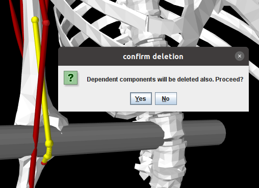
There are situations where one may wish to remove a component but not the components that depend on it. For example, if one wishes to replace a rigid body with a different rigid body, or an FEM model of the same structure, one may wish to transfer to the new body the joints and markers that depend on the original body. This is described more in the following section.
12.5.3 Attaching and transferring to ArtiSynth components
New ArtiSynth components can be attached to OpenSim components through the general point and frame attachment mechanisms described in Sections 3.9, 6.4, and 6.6.
Contact behaviors (Chapter 8) can also be set between OpenSim and/or ArtiSynth components. When working with the former, it may be desirable to replace body surface meshes (using setSurfaceMesh()), or add additional meshes for collision purposes (using addMesh()).
In some instances, one may wish to transfer OpenSim joints, path points, markers or wrap objects to new ArtiSynth components. For joints, one can use the various setBodies() or setBodyA/B() methods described in Section 3.4.3 to reassign one or both bodies for an existing joint.
OpenSim wrap objects are attached to their parent bodies using a frame attachment. Attaching to a different body involves replacing this attachment. However, when doing so, the existing frame attachment must be removed and the existing wrap object should probably be removed from its parent body and placed elsewhere in the component hierarchy. To make this easier, OpenSimParser supplies the method removeWrapObject() that disconnects a wrap object from its parent body and removes its attachment; the application can then move the wrap object elsewhere and reattach it:
For transferring markers and path points to other bodies, OpenSimParser supplies the methods
| Marker replacePathPoint (PointSpringBase muscle, Marker pnt, PointAttachable body) | |
| Marker replaceMarker (Marker mkr, PointAttachable body) | |
replacePathPoint() replaces the path point pnt of the specified muscle with a new point (also implemented as a Marker, though not necessarily a FrameMarker) attached to the specified body. The new point is placed in the same location of the muscle as the original. Similarly, replaceMarker() replaces the marker mkr within the marker set with a new marker attached to the specified body.
12.5.4 Example: replacing the elbow joint with a contact FEM model
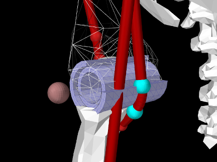
The model
artisynth.demos.opensim.Arm26FemElbow
presents a modified version of OpenSimArm26 in which the elbow joint has been removed and replaced with a (very simple) contact model involving two nested FEM cylinders simulating cartilage layers, with the outer layer attached to the lower arm and the inner one attached to the humerus (Figure 12.6). Additional stability is supplied by a FrameSpring, located where the elbow joint was, that prevents sliding and limits rotation along and about the joint axis. The class definition, excluding import statements, is shown below:
In the build() method, super.build() is first called to create the OpenSimArm26 model which this example extends. Then the geometry folder is located relative to the model’s source folder (line 25), and the humerus, lower arm, and elbow components are located using the parser’s findBody() and findJoint() methods (lines 25-30).
The FEM models used to simulate the inner and outer cartilage layers are defined with respect to the elbow’s D frame, which is located in world coordinates using its getCurrentTDW() method (line 35). The models themselves, which are defined as Gmsh files in the geometry folder, are read using GmshReader (Section 6.2.2), initialized with the helper method initializeFem() which sets their material and rendering properties (lines 5-19), transformed to the D frame, and added to the MechModel (lines 40-48). The inner and outer layers are then connected to the humerus and lower arm, respectively, by attaching nodes whose numbers are specified by node number files (Section 6.4.6) also located in the geometry folder (lines 52-60).
With the cartilage models connected, the elbow joint is removed (line 64). It
is replaced by a FrameSpring (lines 65-74) to supply the stabilization
effected by other tissues surrounding the joint. The spring is centered on the
D frame, and uses a PowerFrameMaterial
(Section 3.7.2.1) with all stiffnesses set to 0 except for
a translational stiffness along ![]() to limit sliding along the joint axis, and
a rotational stiffness (with a deadband of
to limit sliding along the joint axis, and
a rotational stiffness (with a deadband of ![]() ) about
) about ![]() to limit joint axis
rotation to the approximate range
to limit joint axis
rotation to the approximate range ![]() .
.
Note the use of setUseTransformDC(false) when setting up the FrameSpring. As described in Section 3.7.1, this makes the spring compute its restoring forces using
Frictionless contact is enabled between the cartilage models (lines 77-78), and to improve stability this contact is made compliant (Section 8.7.1, lines 80-82) and the model’s step size is decreased to 0.005 sec (line 83).
Removal of the elbow joint revealed that the quiescent forces in the muscles "BIClong" and "BRA" were large enough to cause a large upward impulse at the start of the simulation. To eliminate this, the tendon slack length for these muscles is reset to equal the difference between the total muscle length and the optimal fibre length (lines 87-91; this calculation uses the fact that the optimal pennation angle is 0). To further reduce initial forces, the bias excitations present in the OpenSim model are also removed (line 93). Finally, to enable the FEM joint to be seen, the wrap object "TRI" is made invisible (line 96).
To run this example in ArtiSynth, select All demos > opensim > Arm26FemElbow from the Models menu.
It is possible to make this model go unstable, usually with an “inverted elements” error, if sufficiently large or abrupt forces are exerted on it via the pull controller or the excitation panel.
12.5.5 Example: replacing the humerus with a FEM model
The model
artisynth.demos.opensim.Arm26FemHumerus
presents a modified version of OpenSimArm26 in which the humerus has been replaced with an FEM model, with the joints, wrap objects, and muscle path points transferred from the humerus body to the FEM model (Figure 12.7). Most of this transfer is based on three Frame objects that are attached to the top, middle and center of the FEM model, using the methods described in Section 6.6. These frames serve as anchors for attaching the shoulder and elbow joints, the wrap objects, and the muscle path points that are far enough from the FEM that direct point-to-FEM connections are problematic. Forces applied to wrap objects and path points are transmitted to the FEM model via the frames, which are given a large number of supporting nodes so that the resulting stresses are distributed across a reasonable number of elements.
The build() method for Arm26FemHumerus makes use of the following helper methods:
nearestFrame() finds the frame whose origin is nearest to a given
position vector. createFrameAttachment() creates a FrameFem3dAttachment (Section 6.6) for a frame
located at the pose described by TFW and supported by a set of nodes that
are within a prescribed distance of the frame’s ![]() axis. This choice of
supporting nodes is based on the fact that much of the force in this model
involves moments about the
axis. This choice of
supporting nodes is based on the fact that much of the force in this model
involves moments about the ![]() axis, but other choices are possible. The
critical point is to choose enough nodes so that stresses induced by frame forces
are distributed reasonably well within the model. The method addFemFrame() creates a Frame object initially located at
TFW, gives it a name, and attaches it to a FEM model using an
attachment created by createFrameAttachment().
axis, but other choices are possible. The
critical point is to choose enough nodes so that stresses induced by frame forces
are distributed reasonably well within the model. The method addFemFrame() creates a Frame object initially located at
TFW, gives it a name, and attaches it to a FEM model using an
attachment created by createFrameAttachment().
The build() method itself is listed below:
First, super.build() is called to create the OpenSimArm26 model which this example extends. The parser’s findBody() method is then used to locate the humerus body that is being replaced (line 45).
The FEM model replacing the humerus body is created and added to the MechModel at lines (47-66). A tetrahedral element mesh is created from a surface mesh (read from a geometry directory) by FemFactory.createFromMesh(). Material properties are assigned, with the FEM model given the same density as that of the humerus body (which is higher than bone density to account for the mass of surrounding tissue). Since the defining surface mesh uses the same coordinate system as the original humerus mesh, the model geometry can be transformed into the correct position using the pose of the humerus body (line 59).
The remainder of the build() method transfers the joints, wrap objects, muscle path points and markers from the humerus body to the FEM model. Joints are transferred at lines 60-76. The humerus corresponds to body A of the shoulder joint and body B of the elbow joint, and so setBodyA() and setBodyB() are used, respectively, to reconnect these to the FEM model at the shoulder’s C frame and the elbow’s D frame. Attachments are generated by createFrameAttachment(), using the world locations of the C and D frames returned by the joint methods getCurrentTCW() and getCurrentTDW().
At lines 81-88, addFemFrame() is used to create and attach three anchoring frames to the top, middle and bottom of the FEM model. The top and bottom frames are located at the C and D frames of the shoulder and elbow joints, while the middle frame is placed at an offset from the C frame. All wrap objects connected to the humerus body are reconnected to one of these frames (lines 91-100). For each wrap object, the parser’s removeWrapObject() removes it from the OpenSim component hierarchy and deletes its attachment, the object is cast to a RigidBody and added to the MechModel’s default rigid body list (other locations could be used), and a new attachment is created between the wrap object and the nearest anchor frame.
The muscle path points are transferred at lines 104-123. The code iterates through all the points of all the muscles. Since OpenSimParser implements all path points as FrameMarkers, each point can be cast to a FrameMarker and inspected to see if its frame is the original humerus body. If it is, the point must be replaced with a new marker attached to the FEM model. If the point is either the first or last path point, then it is an origin or insertion and so is near enough to the FEM model that it can be attached directly. Otherwise, it is attached to the nearest anchor frame. Point replacement is performed by the parser’s replacePathPoint() method.
Lastly, the "r_humerus_epicondyle" marker is transferred to the bottom anchor frame, using the parser’s replaceMarker() method, and the humerus body is removed from the body set. There is no need to do this removal using the ComponentUtils method deleteComponentAndDependencies() since all dependencies have been removed by the preceding steps.
To run this example in ArtiSynth, select All demos > opensim > Arm26FemHumerus from the Models menu.
Chapter 13 DICOM Images
Some models are derived from image data, and it may be useful to show the model and image in the same space. For this purpose, a DICOM image widget has been designed, capable of displaying 3D DICOM volumes as a set of three perpendicular planes. An example widget and its property panel is shown in Figure 13.1.
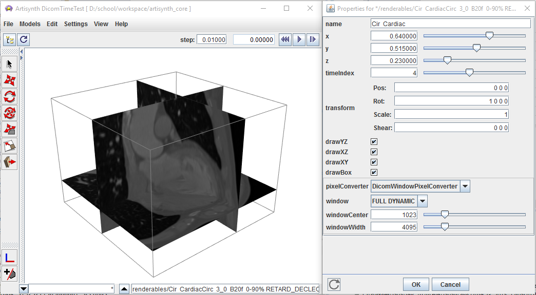
The main classes related to the reading and displaying of DICOM images are:
-
Describes a single attribute in a DICOM file.
Contains all header attributes (all but the image data) extracted from a DICOM file.
Contains the decoded image pixels for a single image frame.
Contains both the header and image information for a single 2D DICOM slice.
Container for DICOM slices, creating a 3D volume (or 3D + time)
Parses DICOM files and folders, appending information to a DicomImage.
Displays the DicomImage in the viewer.
If the purpose is simply to display a DICOM volume in the ArtiSynth viewer, then only the last three classes will be of interest. Readers who simply want to display a DICOM image in their model can skip to Section 13.3.
13.1 The DICOM file format
For a complete description of the DICOM format, see the specification page at
which provides a brief description. Another excellent resource is the blog by Roni Zaharia:
Each DICOM file contains a number of concatenated attributes (a.k.a. elements), one of which defines the embedded binary image pixel data. The other attributes act as meta-data, which can contain identity information of the subject, equipment settings when the image was acquired, spatial and temporal properties of the acquisition, voxel spacings, etc.... The image data typically represents one or more 2D images, concatenated, representing slices (or ‘frames’) of a 3D volume whose locations are described by the meta-data. This image data can be a set of raw pixel values, or can be encoded using almost any image-encoding scheme (e.g. JPEG, TIFF, PNG). For medical applications, the image data is typically either raw or compressed using a lossless encoding technique. Complete DICOM acquisitions are typically separated into multiple files, each defining one or few frames. The frames can then be assembled into 3D image ‘stacks’ based on the meta-information, and converted into a form appropriate for display.
| VR | Description |
|---|---|
| CS | Code String |
| DS | Decimal String |
| DT | Date Time |
| IS | Integer String |
| OB | Other Byte String |
| OF | Other Float String |
| OW | Other Word String |
| SH | Short String |
| UI | Unique Identifier |
| US | Unsigned Short |
| OX | One of OB, OW, OF |
Each DICOM attribute is composed of:
-
•
a standardized unique integer tag in the format (XXXX,XXXX) that defines the group and element of the attribute
-
•
a value representation (VR) that describes the data type and format of the attribute’s value (see Table 13.1)
-
•
a value length that defines the length in bytes of the attribute’s value to follow
-
•
a value field that contains the attribute’s value
This layout is depicted in Figure 13.2. A list of important attributes are provided in Table 13.2.
| Tag | VR | Value Length | Value Field |
| Attribute name | VR | Tag | |
|---|---|---|---|
| Transfer syntax UID | UI | 0x0002 , | 0x0010 |
| Slice thickness | DS | 0x0018 , | 0x0050 |
| Spacing between slices | DS | 0x0018 , | 0x0088 |
| Study ID | SH | 0x0020 , | 0x0010 |
| Series number | IS | 0x0020 , | 0x0011 |
| Acquisition number | IS | 0x0020 , | 0x0012 |
| Image number | IS | 0x0020 , | 0x0013 |
| Image position patient | DS | 0x0020 , | 0x0032 |
| Image orientation patient | DS | 0x0020 , | 0x0037 |
| Temporal position identifier | IS | 0x0020 , | 0x0100 |
| Number of temporal positions | IS | 0x0020 , | 0x0105 |
| Slice location | DS | 0x0020 , | 0x1041 |
| Samples per pixel | US | 0x0028 , | 0x0002 |
| Photometric interpretation | CS | 0x0028 , | 0x0004 |
| Planar configuration (color) | US | 0x0028 , | 0x0006 |
| Number of frames | IS | 0x0028 , | 0x0008 |
| Rows | US | 0x0028 , | 0x0010 |
| Columns | US | 0x0028 , | 0x0011 |
| Pixel spacing | DS | 0x0028 , | 0x0030 |
| Bits allocated | US | 0x0028 , | 0x0100 |
| Bits stored | US | 0x0028 , | 0x0101 |
| High bit | US | 0x0028 , | 0x0102 |
| Pixel representation | US | 0x0028 , | 0x0103 |
| Pixel data | OX | 0x7FE0 , | 0x0010 |
13.2 The DICOM classes
Each DicomElement represents a single attribute contained in a DICOM file. The DicomHeader contains the collection of DicomElements defined in a file, apart from the pixel data. The image pixels are decoded and stored in a DicomPixelBuffer. Each DicomSlice contains a DicomHeader, as well as the decoded DicomPixelBuffer for a single slice (or ‘frame’). All slices are assembled into a single DicomImage, which can be used to extract 3D voxels and spatial locations from the set of slices. These five classes are described in further detail in the following sections.
13.2.1 DicomElement
The DicomElement class is a simple container for DICOM attribute information. It has three main properties:
-
•
an integer tag
-
•
a value representation (VR)
-
•
a value
These properties can be obtained using the corresponding get function: getTag(), getVR(), getValue(). The tag refers to the concatenated group/element tag. For example, the transfer syntax UID which corresponds to group 0x0002 and element 0x0010 has a numeric tag of 0x00020010. The VR is represented by an enumerated type, DicomElement.VR. The ‘value’ is the raw value extracted from the DICOM file. In most cases, this will be a String. For raw numeric values (i.e. stored in the DICOM file in binary form) such as the unsigned short (US), the ‘value’ property is exactly the numeric value.
For VRs such as the integer string (IS) or decimal string (DS), the string will still need to be parsed in order to extract the appropriate sequence of numeric values. There are static utility functions for handling this within DicomElement. For a ‘best-guess’ of the desired parsed value based on the VR, one can use the method getParsedValue(). Often, however, the desired value is also context-dependent, so the user should know a priori what type of value(s) to expect. Parsing can also be done automatically by querying for values directly through the DicomHeader object.
13.2.2 DicomHeader
When a DICOM file is parsed, all meta-data (attributes apart from the actual pixel data) is assembled into a DicomHeader object. This essentially acts as a map that can be queried for attributes using one of the following methods:
The first method returns the full element as described in the previous section. The remaining methods are used for convenience when the desired value type is known for the given tag. These methods automatically parse or convert the DicomElement’s value to the desired form.
If the tag does not exist in the header, then the getIntValue(...) and getDecimalValue(...) will return the supplied defaultValue. All other methods will return null.
13.2.3 DicomPixelBuffer
The DicomPixelBuffer contains the decoded image information of an image slice. There are three possible pixel types currently supported:
-
•
byte grayscale values (PixelType.BYTE)
-
•
short grayscale values (PixelType.SHORT)
-
•
byte RGB values, with layout RGBRGB...RGB (PixelType.BYTE_RGB)
The pixel buffer stores all pixels in one of these types. The pixels can be queried for directly using getPixel(idx) to get a single pixel, or getBuffer() to get the entire pixel buffer. Alternatively, a DicomPixelInterpolator object can be passed in to convert between pixel types via one of the following methods:
These methods populate an output array or buffer with converted pixel values, which can later be passed to a renderer. For further details on these methods, refer to the Javadoc documentation.
13.2.4 DicomSlice
A single DICOM file contains both header information, and one or more image ‘frames’ (slices). In ArtiSynth, we separate each frame and attach them to the corresponding header information in a DicomSlice. Thus, each slice contains a single DicomHeader and DicomPixelBuffer. These can be obtained using the methods: getHeader() and getPixelBuffer().
For convenience, the DicomSlice also has all the same methods for extracting and converting between pixel types as the DicomPixelBuffer.
13.2.5 DicomImage
A complete DICOM acquisition typically consists of multiple slices forming a 3D image stack, and potentially contains multiple 3D stacks to form a dynamic 3D+time image. The collection of DicomSlices are thus assembled into a DicomImage, which keeps track of the spatial and temporal positions.
The DicomImage is the main object to query for pixels in 3D(+time). To access pixels, it has the following methods:
The inputs {x, y, z} refer to voxel indices, and time refers to the time instance index, starting at zero. The four voxel dimensions of the image can be queried with: getNumCols() getNumRows(), getNumSlices(), and getNumTimes().
The DicomImage also contains spatial transform information for converting between voxel indices and patient-centered spatial locations. The affine transform can be acquired with the method getPixelTransform(). This allows the image to be placed in the appropriate 3D location, to correspond with any derived data such as segmentations. The spatial transformation is automatically extracted from the DICOM header information embedded in the files.
13.3 Loading a DicomImage
DICOM files and folders are read using the DicomReader class. The reader populates a supplied DicomImage with slices, forming the full 3D(+time) image. The basic pattern is as follows:
The first argument in the read(...) command is an existing image in which to append slices. In this case, we pass in null to signal that a new image is to be created.
In some cases, we might wish to exclude certain files, such as meta-data files that happen to be in the DICOM folder. By default, the reader attempts to read all files in a given directory, and will print out an error message for those it fails to detect as being in a valid DICOM format. To limit the files to be considered, we allow the specification of a Java Pattern, which will test each filename against a regular expression. Only files with names that match the pattern will be included. For example, in the following, we limit the reader to files ending with the “dcm” extension.
The pattern is applied to the absolute filename, with either windows and mac/linux file separators (both are checked against the regular expression). The method also has an option to recursively search for files in subdirectories. If the full list of files is known, then one can use the method:
which will load all specified files.
13.3.1 Time-dependent images
In most cases, time-dependent images will be properly assembled using the previously mentioned methods in the DicomReader. Each slice should have a temporal position identifier that allows for the separate image stacks to be separated. However, we have found in practice that at times, the temporal position identifier is omitted. Instead, each stack might be stored in a separate DICOM folder. For this reason, additional read methods have been added that allow manual specification of the time index:
If the supplied temporalPosition is non-negative, then the temporal position of all included files will be manually set to that value. If negative, then the method will attempt to read the temporal position from the DICOM header information. If no such information is available, then the reader will guess the temporal position to be one past the last temporal position in the original image stack (or 0 if im == null). For example, if the original image has temporal positions {0, 1, 2}, then all appended slices will have a temporal position of three.
13.3.2 Image formats
The DicomReader attempts to automatically decode any pixel information embedded in the DICOM files. Unfortunately, there are virtually an unlimited number of image formats allowed in DICOM, so there is no way to include native support to decode all of them. By default, the reader can handle raw pixels, and any image format supported by Java’s ImageIO framework, which includes JPEG, PNG, BMP, WBMP, and GIF. Many medical images, however, rely on lossless or near-lossless encoding, such as lossless JPEG, JPEG 2000, or TIFF. For these formats, we provide an interface that interacts with the third-party command-line utilities provided by ImageMagick (http://www.imagemagick.org). To enable this interface, the ImageMagick utilities identify and convert must be available and exist somewhere on the system’s PATH environment variable.
ImageMagick Installation
To enable ImageMagick decoding, required for image formats not natively supported by Java (e.g. JPEG 2000, TIFF), download and install the ImageMagick command-line utilities from: http://www.imagemagick.org/script/binary-releases.php
The install path must also be added to your system’s PATH environment variable so that ArtiSynth can locate the identify and convert utilities.
13.4 The DicomViewer
Once a DicomImage is loaded, it can be displayed in a model by using the DicomViewer component. The viewer has several key properties:
- name
-
the name of the viewer component
- x, y, z
-
the normalized slice positions, in the range [0,1], at which to display image planes
- timeIndex
-
the temporal position (image stack) to display
- transform
-
an affine transformation to apply to the image (on top of the voxel-to-spatial transform extracted from the DICOM file)
- drawYZ
-
draw the YZ plane, corresponding to position x
- drawXZ
-
draw the XZ plane, corresponding to position y
- drawXY
-
draw the XY plane, corresponding to position z
- drawBox
-
draw the 3D image’s bounding box
- pixelConverter
-
the interpolator responsible for converting pixels decoded in the DICOM slices into values appropriate for display. The converter has additional properties:
- window
-
name of a preset window for linear interpolation of intensities
- center
-
center intensity
- width
-
width of window
Each property has a corresponding getXxx(...) and setXxx(...) method that can adjust the settings in code. They can also be modified directly in the ArtiSynth GUI. The last property, the pixelConverter allows for shifting and scaling intensity values for display. By default a set of intensity ‘windows’ are loaded directly from the DICOM file. Each window has a name, and defines a center and width used to linearly scale the intensity range. In addition to the windows extracted from the DICOM, two new windows are added: FULL_DYNAMIC, corresponding to the entire intensity range of the image; and CUSTOM, which allows for custom specification of the window center and width properties.
To add a DicomViewer to the model, create the viewer by supplying a component name and reference to a DicomImage, then add it as a Renderable to the RootModel:
The image will automatically be displayed in the patient-centered coordinates loaded from the DicomImage. In addition to this basic construction, there are convenience constructors to avoid the need for a DicomReader for simple DICOM files:
These constructors generate a new DicomImage internal to the viewer. The image can be retrieved from the viewer using the getImage() method.
13.5 DICOM example
Some examples of DICOM use can be found in the artisynth.demos.dicom package. The model DicomTest loads a partial image of a heart, which is initially downloaded from the ArtiSynth website:
Lines 23-28 are responsible for downloading and extracting the sample DICOM zip file. In the end, dicomPath contains a reference to the desired DICOM file on the local system, which is used to create a viewer on line 34. We then add the viewer to the model for display purposes.
To run this example in ArtiSynth, select All demos > dicom > DicomTest from the Models menu. The model should load and initially appear as in Figure 13.3.
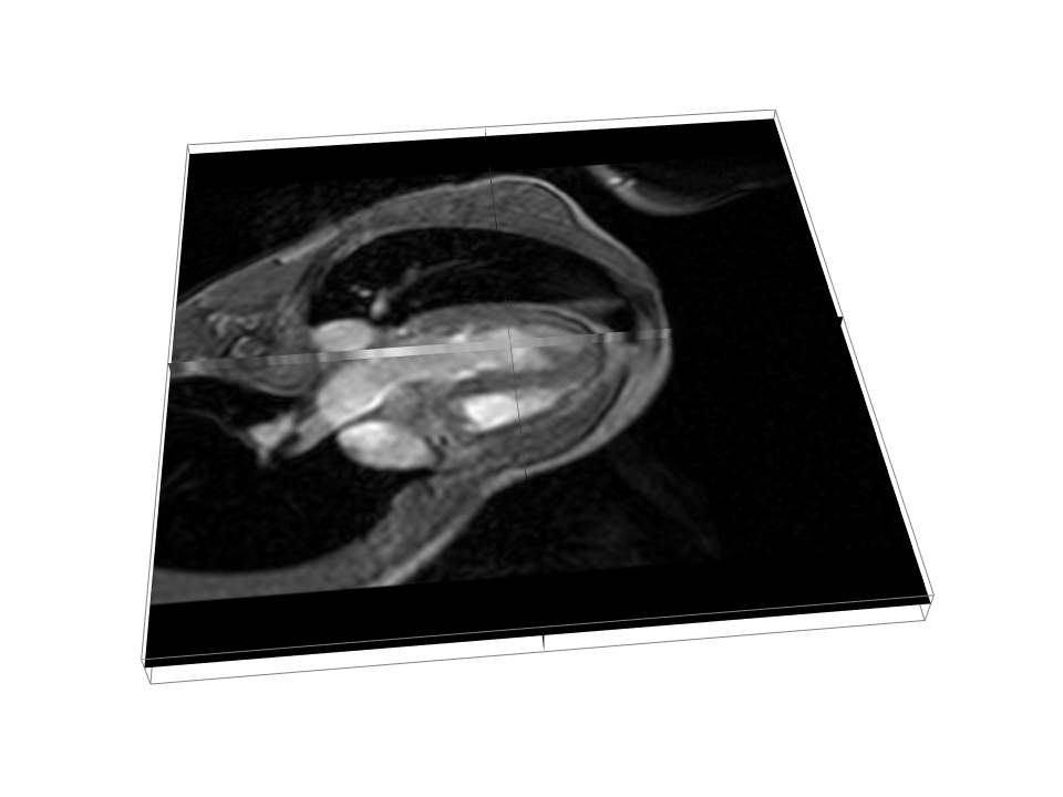
Appendix A Mathematical Review
This appendix reviews some of the mathematical concepts used in this manual.
A.1 Rotation transforms
Rotation matrices are used to describe the orientation of 3D coordinate frames in space, and to transform vectors between these coordinate frames.

Consider two 3D coordinate frames A and B that are rotated with
respect to each other (Figure A.1). The orientation
of B with respect to A can be described by a ![]() rotation
matrix
rotation
matrix ![]() , whose columns are the unit vectors giving the
directions of the rotated axes
, whose columns are the unit vectors giving the
directions of the rotated axes ![]() ,
, ![]() , and
, and ![]() of B with
respect to A.
of B with
respect to A.
![]() is an orthogonal matrix, meaning that
its columns are both of unit length and mutually
orthogonal, so that
is an orthogonal matrix, meaning that
its columns are both of unit length and mutually
orthogonal, so that
| (A.1) |
where ![]() is the
is the ![]() identity matrix. The inverse
of
identity matrix. The inverse
of ![]() is hence equal to its transpose:
is hence equal to its transpose:
| (A.2) |
Because ![]() is orthogonal,
is orthogonal, ![]() , and because it
is a rotation,
, and because it
is a rotation, ![]() (the other case, where
(the other case, where ![]() , is not a rotation but a reflection). The 6 orthogonality
constraints associated with a rotation matrix mean that in spite of
having 9 numbers, the matrix only has 3 degrees of freedom.
, is not a rotation but a reflection). The 6 orthogonality
constraints associated with a rotation matrix mean that in spite of
having 9 numbers, the matrix only has 3 degrees of freedom.
Now, assume we have a 3D vector ![]() , and consider its coordinates
with respect to both frames A and B. Where necessary, we use a
preceding superscript to indicate the coordinate frame with respect to
which a quantity is described, so that
, and consider its coordinates
with respect to both frames A and B. Where necessary, we use a
preceding superscript to indicate the coordinate frame with respect to
which a quantity is described, so that ![]() and
and ![]() denote
denote ![]() with respect to frames A and B, respectively. Given the
definition of
with respect to frames A and B, respectively. Given the
definition of ![]() given above, it is fairly straightforward to
show that
given above, it is fairly straightforward to
show that
| (A.3) |
and, given (A.2), that
| (A.4) |
Hence in addition to describing the orientation of B with respect to A,
![]() is also a transformation matrix that maps vectors in B
to vectors in A.
is also a transformation matrix that maps vectors in B
to vectors in A.
It is straightforward to show that
| (A.5) |

A simple rotation by an angle ![]() about one of the basic
coordinate axes is known as a basic rotation. The three
basic rotations about x, y, and z are:
about one of the basic
coordinate axes is known as a basic rotation. The three
basic rotations about x, y, and z are:
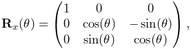 |
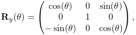 |
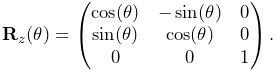 |
Next, we consider transform composition. Suppose we have three
coordinate frames, A, B, and C, whose orientations are related to each other by
![]() ,
, ![]() , and
, and ![]() (Figure
A.2). If we know
(Figure
A.2). If we know ![]() and
and ![]() ,
then we can determine
,
then we can determine ![]() from
from
| (A.6) |
This can be understood in terms of vector transforms. ![]() transforms a vector from C to B, which is equivalent to first
transforming from C to A,
transforms a vector from C to B, which is equivalent to first
transforming from C to A,
| (A.7) |
and then transforming from A to B:
| (A.8) |
Note also from (A.5) that ![]() can be
expressed as
can be
expressed as
| (A.9) |
In addition to specifying rotation matrix components explicitly, there are numerous other ways to describe a rotation. Three of the most common are:
- Roll-pitch-yaw angles
-
There are 6 variations of roll-pitch-yaw angles. The one used in ArtiSynth corresponds to older robotics texts (e.g., Paul, Spong) and consists of a roll rotation
about the z axis, followed by a pitch
rotation  about the new y axis, followed by a yaw rotation
about the new x axis. The net rotation can be expressed by the
following product of basic rotations:
about the new y axis, followed by a yaw rotation
about the new x axis. The net rotation can be expressed by the
following product of basic rotations: 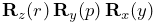 .
. - Axis-angle
-
An axis angle rotation parameterizes a rotation as a rotation by an angle
about a specific axis  . Any rotation
can be represented in such a way as a consequence of Euler’s rotation
theorem.
. Any rotation
can be represented in such a way as a consequence of Euler’s rotation
theorem. - Euler angles
-
There are 6 variations of Euler angles. The one used in ArtiSynth consists of a rotation
about the z axis, followed by a rotation
about the new y axis, followed by a rotation  about the
new z axis. The net rotation can be expressed by the following product
of basic rotations:
about the
new z axis. The net rotation can be expressed by the following product
of basic rotations: 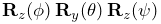 .
.
A.2 Rigid transforms
Rigid transforms are used to specify both the transformation of points and vectors between coordinate frames, as well as the relative position and orientation between coordinate frames.

Consider two 3D coordinate frames in space, A and B (Figure
A.3). The translational position of B with respect to A
can be described by a vector ![]() from the origin of A to the
origin of B (described with respect to frame A). Meanwhile, the
orientation of B with respect to A can be described by the
from the origin of A to the
origin of B (described with respect to frame A). Meanwhile, the
orientation of B with respect to A can be described by the ![]() rotation matrix
rotation matrix ![]() (Section A.1). The
combined position and orientation of B with respect to A is known as
the pose of B with respect to A.
(Section A.1). The
combined position and orientation of B with respect to A is known as
the pose of B with respect to A.

Now, assume we have a 3D point ![]() , and consider its coordinates with
respect to both frames A and B (Figure A.4). Given the
pose descriptions given above, it is fairly straightforward to show
that
, and consider its coordinates with
respect to both frames A and B (Figure A.4). Given the
pose descriptions given above, it is fairly straightforward to show
that
| (A.10) |
and, given (A.2), that
| (A.11) |
If we extend our points into a 4D homogeneous coordinate space
with the fourth coordinate ![]() equal to 1, i.e.,
equal to 1, i.e.,
| (A.12) |
then (A.10) and (A.11) can be simplified to
where
| (A.13) |
and
| (A.14) |
![]() is the
is the ![]() rigid transform matrix that
transforms points from B to A and also describes the pose of
B with respect to A (Figure A.5).
rigid transform matrix that
transforms points from B to A and also describes the pose of
B with respect to A (Figure A.5).

It is straightforward to show that ![]() and
and ![]() describe the orientation and position of
describe the orientation and position of ![]() with respect to
with respect to
![]() , and so therefore
, and so therefore
| (A.15) |
Note that if we are transforming a vector ![]() instead of a point
between B and A, then we are only concerned about relative orientation
and the vector transforms (A.3) and
(A.4) should be used instead.
However, we can express these using
instead of a point
between B and A, then we are only concerned about relative orientation
and the vector transforms (A.3) and
(A.4) should be used instead.
However, we can express these using ![]() if
we embed vectors in a homogeneous coordinate space
with the fourth coordinate
if
we embed vectors in a homogeneous coordinate space
with the fourth coordinate ![]() equal to 0, i.e.,
equal to 0, i.e.,
| (A.16) |
so that

A.3 Affine transforms
An affine transform is a generalization of a rigid transform, in
which the rotational component ![]() is replaced by a general
is replaced by a general ![]() matrix
matrix ![]() . This means that an affine transform implements a
generalized basis transformation combined with an offset of the origin
(Figure A.7). As with
. This means that an affine transform implements a
generalized basis transformation combined with an offset of the origin
(Figure A.7). As with ![]() for rigid transforms, the
columns of
for rigid transforms, the
columns of ![]() still describe the transformed basis vectors
still describe the transformed basis vectors ![]() ,
,
![]() , and
, and ![]() , but these are generally no longer orthonormal.
, but these are generally no longer orthonormal.

Expressed in terms of homogeneous coordinates,
the affine transform ![]() takes the form
takes the form
| (A.18) |
with
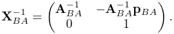 |
(A.19) |
As with rigid transforms, when an affine transform is applied to a
vector instead of a point, only the matrix ![]() is applied and the
translation component
is applied and the
translation component ![]() is ignored.
is ignored.
Affine transforms are typically used to effect transformations that
require stretching and shearing of a coordinate frame. By the polar
decomposition theorem, ![]() can be factored into a regular
rotation
can be factored into a regular
rotation ![]() plus a symmetric shearing/scaling matrix
plus a symmetric shearing/scaling matrix ![]() :
:
| (A.20) |
Affine transforms can also be used to perform reflections, in which
![]() is orthogonal (so that
is orthogonal (so that ![]() ) but with
) but with ![]() .
.
A.4 Rotational velocity

Given two 3D coordinate frames A and B, the rotational, or angular, velocity of B with respect to A is given by a 3D vector
![]() (Figure A.8).
(Figure A.8). ![]() is related to the derivative of
is related to the derivative of ![]() by
by
| (A.21) |
where ![]() and
and ![]() indicate
indicate ![]() with
respect to frames
with
respect to frames ![]() and
and ![]() and
and ![]() denotes the
denotes the ![]() cross product matrix
cross product matrix
![[\boldsymbol{\omega}]\equiv\left(\begin{matrix}0&-\omega_{z}&\omega_{y}\\
\omega_{z}&0&-\omega_{x}\\
-\omega_{y}&\omega_{x}&0\\
\end{matrix}\right).](mi/mi1790.png) |
(A.22) |
If we consider instead the velocity of ![]() with respect to
with respect to ![]() , it is
straightforward to show that
, it is
straightforward to show that
| (A.23) |
A.5 Spatial velocities and forces
Given two 3D coordinate frames A and B, the spatial velocity,
or twist,
![]() of B with respect to A is given by the 6D
composition of the translational velocity
of B with respect to A is given by the 6D
composition of the translational velocity ![]() of the
origin of B with respect to A and the angular velocity
of the
origin of B with respect to A and the angular velocity ![]() :
:
| (A.24) |
Similarly, the spatial force, or wrench, ![]() acting
on a frame B is given by the 6D composition of the translational force
acting
on a frame B is given by the 6D composition of the translational force
![]() acting on the frame’s origin and the moment
acting on the frame’s origin and the moment ![]() , or torque,
acting through the frame’s origin:
, or torque,
acting through the frame’s origin:
| (A.25) |
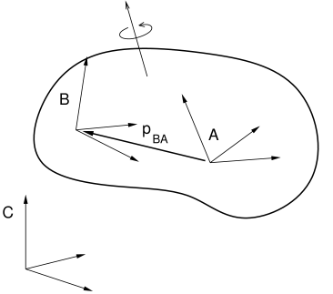
If we have two frames ![]() and
and ![]() rigidly connected within a rigid
body (Figure A.9), and we know the spatial velocity
rigidly connected within a rigid
body (Figure A.9), and we know the spatial velocity
![]() of
of ![]() with respect to some third frame
with respect to some third frame ![]() , we may wish
to know the spatial velocity
, we may wish
to know the spatial velocity ![]() of
of ![]() with respect to
with respect to ![]() .
The angular velocity components are the same, but the translational
velocity components are coupled by the angular velocity and the offset
.
The angular velocity components are the same, but the translational
velocity components are coupled by the angular velocity and the offset
![]() between
between ![]() and
and ![]() , so that
, so that
![]() is hence related to
is hence related to ![]() via
via
where ![]() is defined by
(A.22).
is defined by
(A.22).
The above equation assumes that all quantities are expressed
with respect to the same coordinate frame.
If we instead consider ![]() and
and ![]() to be represented
in frames
to be represented
in frames ![]() and
and ![]() , respectively, then
we can show that
, respectively, then
we can show that
| (A.26) |
where
| (A.27) |
The transform ![]() is easily formed from the components of the
rigid transform
is easily formed from the components of the
rigid transform ![]() relating
relating ![]() to
to ![]() .
.
The spatial forces ![]() and
and ![]() acting on frames
acting on frames ![]() and
and
![]() within a rigid body are related in a similar way, only with
spatial forces, it is the moment that is coupled through the moment
arm created by
within a rigid body are related in a similar way, only with
spatial forces, it is the moment that is coupled through the moment
arm created by ![]() , so that
, so that
If we again assume that ![]() and
and ![]() are expressed in frames
are expressed in frames ![]() and
and ![]() , we can show that
, we can show that
| (A.28) |
where
| (A.29) |
A.6 Spatial inertia
Assume we have a rigid body with mass ![]() and a coordinate frame
located at the body’s center of mass. If
and a coordinate frame
located at the body’s center of mass. If ![]() and
and ![]() give the
translational and rotational velocity of the coordinate frame, then
the body’s linear and angular momentum
give the
translational and rotational velocity of the coordinate frame, then
the body’s linear and angular momentum ![]() and
and ![]() are given by
are given by
| (A.30) |
where ![]() is the
is the ![]() rotational inertia with respect
to the center of mass. These relationships can be combined into a
single equation
rotational inertia with respect
to the center of mass. These relationships can be combined into a
single equation
| (A.31) |
where ![]() is the spatial momentum and
is the spatial momentum and ![]() is a
is a ![]() matrix representing the spatial inertia:
matrix representing the spatial inertia:
| (A.32) |
The spatial momentum satisfies Newton’s second law, so that
| (A.33) |
which can be used to find the acceleration of a body in response to a spatial force.
When the body coordinate frame is not located at the center of mass, then the spatial inertia assumes the more complicated form
| (A.34) |
where ![]() is the center of mass and
is the center of mass and ![]() is defined by
(A.22).
is defined by
(A.22).
Like the rotational inertia, the spatial inertia is always symmetric
positive definite if ![]() .
.
Bibliography
- [1] (2002) A time-stepping method for stiff multibody dynamics with contact and friction. International Journal for Numerical Methods in Engineering 55 (7), pp. 753–784. Cited by: §8.9.4.
- [2] (1993) A three-dimensional constitutive model for the large stretch behavior of rubber elastic materials. Journal of the Mechanics and Physics of Solids 41 (2), pp. 389–412. Cited by: §6.10.2.8.
- [3] (2004) Multibody dynamic simulation of knee contact mechanics. Medical engineering & physics 26 (9), pp. 777–789. Cited by: §8.7.3.
- [4] (1991) Ligament-bone interaction in a three-dimensional model of the knee. J. Biomech. Eng. 113 (3), pp. 263–269. Cited by: §4.5.5.3.
- [5] (2005) Three-dimensional representation of complex muscle architectures and geometries. Annals of biomedical engineering 33 (5), pp. 661–673. Cited by: §4.5.1.5, §6.10.3.2, §6.10.3.3, §6.9.3.
- [6] (2000) Nonlinear continuum mechanics for finite element analysis. Cambridge University Press. Cited by: §6.1.
- [7] (2007) OpenSim: open-source software to create and analyze dynamic simulations of movement. IEEE T Bio-Med Eng 54 (11), pp. 1940–1950. Cited by: §1.2.2, §10.1, §10.2.9, §12.1, §4.5.4.1, §4.5.4.2, §4.5.5.3.
- [8] (2008) Geometric skinning with approximate dual quaternion blending. ACM Transactions on Graphics (TOG) 27 (4), pp. 1–23. Cited by: item DUAL_QUATERNION_LINEAR, item DUAL_QUATERNION_ITERATIVE.
- [9] (2007) Ghosts and machines: regularized variational methods for interactive simulations of multibodies with dry frictional contacts. Ph.D. Thesis, Umeå University, Department of Computing Science. Cited by: §3.4.9.
- [10] (2007) Ghosts and machines: regularized variational methods for interactive simulations of multibodies with dry frictional contacts. Ph.D. Thesis, Datavetenskap, UmeÂ, Computer Science Dept., Umea University, Sweden. Cited by: §8.9.4.
- [11] (2012) ArtiSynth: a fast interactive biomechanical modeling toolkit combining multibody and finite element simulation. In Soft tissue biomechanical modeling for computer assisted surgery, pp. 355–394. Cited by: §1.2.3, §1.2, §10.1.3, §10.1.3, §3.4.2.
- [12] (2012-01) FEBio: finite elements for biomechanics. Journal of biomechanical engineering 134, pp. 011005. External Links: Document Cited by: §6.1.2.3.
- [13] FEBio theory manual. Note: https://help.febio.org/FEBio/FEBio_tm_2_7 Cited by: §6.1.2.3, §6.10.1.
- [14] (2012) A computationally efficient muscle model. In Summer Bioengineering Conference, pp. 1055–1056. Cited by: §4.5.6.
- [15] (2013) Flexing computational muscle: modeling and simulation of musculotendon dynamics. Journal of biomechanical engineering 135 (2). Cited by: §4.5.4.1.
- [16] (2004) Interactive virtual materials.. In Graphics interface, Vol. 2004, pp. 239–246. Cited by: §6.1.3, §6.10.1, §6.10.1.
- [17] (2009) Preserving topology and elasticity for embedded deformable models. In ACM Transactions on Graphics (TOG), Vol. 28, pp. 52. Cited by: Chapter 11.
- [18] (2008-02) Efficient deformable body simulation using stiffness-warped nonlinear finite elements. In Symposium on Interactive 3D Graphics and Games (i3D), pp. . Note: poster Cited by: §6.1.3, §6.10.1, §6.10.1.
- [19] (2000) Dynamic simulation of muscle and articular properties during human wide jaw opening. Archives of Oral Biology 45 (11), pp. 963–982. Cited by: §4.5.1.4.
- [20] (2006) A linearly implicit trapezoidal method for integrating stiff multibody dynamics with contact, joints, and friction. International Journal for Numerical Methods in Engineering 66 (7), pp. 1079–1124. Cited by: §8.9.4.
- [21] (2006) Interactive simulation of elastic deformable materials. In Proceedings of SIGRAD Conference 2006 in Skövde, Sweden, pp. 22–32. Cited by: §3.4.9.
- [22] (2011) Simbody: multibody dynamics for biomedical research. Procedia Iutam 2, pp. 241–261. Cited by: §8.7.3.
- [23] (1985) Animating rotation with quaternion curves. In Proceedings of the 12th annual conference on Computer graphics and interactive techniques, pp. 245–254. Cited by: 2nd item.
- [24] (2016) Influence of ligament properties on tibiofemoral mechanics in walking. The journal of knee surgery, pp. 099–106. Cited by: §4.5.5.3.
- [25] (2014) Unified skinning of rigid and deformable models for anatomical simulati on s. In SIGGRAPH Asia 2014 Technical Briefs, pp. 9. Cited by: Figure 11.1, Chapter 11.
- [26] (1995) Curve and surface smoothing without shrinkage. In Computer Vision, 1995. Proceedings., Fifth International Conference on, pp. 852–857. Cited by: §9.3.
- [27] (2003) Adjustment of muscle mechanics model parameters to simulate dynamic contractions in older adults. J. Biomech. Eng. 125 (1), pp. 70–77. Cited by: §4.5.4.2, §4.5.4.2, §4.5.4.2, §4.5.4.2.
- [28] (1970) Mechanical characterization of skin-finite deformations. Journal of biomechanics 3 (1), pp. 111–124. Cited by: §6.10.2.9.
![[LOGO]](data:image/png;base64,iVBORw0KGgoAAAANSUhEUgAAAAsAAAAOCAYAAAD5YeaVAAAAAXNSR0IArs4c6QAAAAZiS0dEAP8A/wD/oL2nkwAAAAlwSFlzAAALEwAACxMBAJqcGAAAAAd0SU1FB9wKExQZLWTEaOUAAAAddEVYdENvbW1lbnQAQ3JlYXRlZCB3aXRoIFRoZSBHSU1Q72QlbgAAAdpJREFUKM9tkL+L2nAARz9fPZNCKFapUn8kyI0e4iRHSR1Kb8ng0lJw6FYHFwv2LwhOpcWxTjeUunYqOmqd6hEoRDhtDWdA8ApRYsSUCDHNt5ul13vz4w0vWCgUnnEc975arX6ORqN3VqtVZbfbTQC4uEHANM3jSqXymFI6yWazP2KxWAXAL9zCUa1Wy2tXVxheKA9YNoR8Pt+aTqe4FVVVvz05O6MBhqUIBGk8Hn8HAOVy+T+XLJfLS4ZhTiRJgqIoVBRFIoric47jPnmeB1mW/9rr9ZpSSn3Lsmir1fJZlqWlUonKsvwWwD8ymc/nXwVBeLjf7xEKhdBut9Hr9WgmkyGEkJwsy5eHG5vN5g0AKIoCAEgkEkin0wQAfN9/cXPdheu6P33fBwB4ngcAcByHJpPJl+fn54mD3Gg0NrquXxeLRQAAwzAYj8cwTZPwPH9/sVg8PXweDAauqqr2cDjEer1GJBLBZDJBs9mE4zjwfZ85lAGg2+06hmGgXq+j3+/DsixYlgVN03a9Xu8jgCNCyIegIAgx13Vfd7vdu+FweG8YRkjXdWy329+dTgeSJD3ieZ7RNO0VAXAPwDEAO5VKndi2fWrb9jWl9Esul6PZbDY9Go1OZ7PZ9z/lyuD3OozU2wAAAABJRU5ErkJggg==)